This page shows how to obtain the results and graphical figures displayed in Hamilton’s Chapter 1 using SAS. Chapter 1 uses the concord1 data. You can copy and paste this data step into the program editor to run the examples below.
Mean, Variance and Standard Deviation
Use the means procedure to get the sample means and standard deviations for 1980 and 1981 water use (pages 2-4).
proc means data=concord1 mean var std n;
  var water81 water80;
run;
The MEANS Procedure
Variable Label                 Mean    Variance   Std Dev N
-------------------------------------------------------------
WATER81  Summer 1981 Water Use 2298.39 2208563.05 1486.12 496
WATER80  Summer 1980 Water Use 2732.06 3110990.51 1763.80 496
-------------------------------------------------------------
Normal Distributions
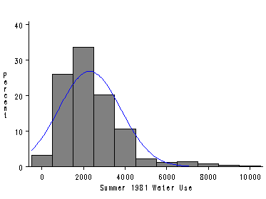
Figure 1.2, page 6. Use the histogram statement with the normal option in proc univariate to graph the plot. The median and percentiles on pages 7-8 are also computed here, but not all the output from the univariate procedure is listed.
proc univariate data=concord1;
   var water81;
   histogram / noframe
               normal(color=blue)
               cfill=GREY
               vaxis=(0 to 40 by 10);
run;
The SAS System
The UNIVARIATE Procedure
Variable: WATER81 (Summer 1981 Water Use)
Moments

N                      496   Sum Weights             496
Mean             2298.3871   Sum Observations    1140000
Std Deviation    1486.1235   Variance         2208563.05
Skewness        1.72754384   Kurtosis         4.71525305
Uncorrected SS  3713400000   Corrected SS     1093238710
Coeff Variation 64.6594083   Std Error Mean   66.7289149

Basic Statistical Measures

Location                 Variability

Mean   2298.387    Std Deviation             1486
Median 2050.000    Variance               2208563
Mode   1000.000    Range                    10000
                   Interquartile Range       1700
Quantiles (Definition 5)
Quantile       Estimate
100% Max          10100
99%                8100
95%                4800
90%                4000
75% Q3             2900
50% Median         2050
25% Q1             1200
10%                 800
5%                  500
1%                  200
0% Min              100
Boxplots
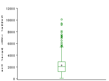
Figure 1.3, page 9. To graph the distribution of only one variable, we must first create a variable which is any constant value. This is not necessary to graph a boxplot of water81 by some other variable.
Create a constant variable called cvar.
data c1;
  set concord1;
  cvar=0;
We create a blank axis called axis2 to use as the horizontal axis, then use proc boxplot.
axis2 label=none value=none major=none minor=none;

proc boxplot data=c1;
    plot water81*cvar / boxstyle=schematic
                        cboxes=green
                        idsymbol=circle
                        noframe
                        haxis=axis2
                        vaxis=(0 to 12000 by 2000);
run;
Symmetry Plots
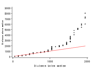
Figure 1.4, page 11. SAS does not have a procedure or graph option to produce a symmetry plot. However, we can compute the distances to points above and below the median to plot the graph manually. Compute the medians and sample sizes and output to a dataset. The statistics for water79 and water80 are also computed here for later use.
proc univariate data=concord1 noprint;
   var water79 water80 water81;
   output out = stats1
          median = med79 med80 med81
          n = n79 n80 n81;
run;
How we calculate the distance above and below the median depends on whether n is even or odd. So we create an even/odd flag which is zero if n is even. This flag, along with the other statistics, are output to global macro variables, accessible in any later data step.
data stats2;
  set stats1;

  evodd81 = mod(n81,2);  /* even/odd flag */

  call symput('evodd81',evodd81);
  call symput('med79',med79);
  call symput('med80',med80);
  call symput('med81',med81);
  call symput('n79',n79);
  call symput('n80',n80);
  call symput('n81',n81);
run;
Sort the data by the variable you wish to plot, keeping only the plot variable to save sorting time and disk space.
proc sort data=concord1
           out=sorted81(keep=water81);
  by water81;
run;
Compute the distances above and below the median and output to two datasets based on whether the points are above or below.
data above81(drop=b)
     below81(drop=a);
  set sorted81;
  i = _n_;

  /* n is even */
  if evodd81 = 0 then do;
     if i <= &n81 / 2 then do;
        b = &med81 - water81;
        output below81;
     end;
     else do;
        a = water81 - &med81;
        output above81;
     end;
  end;

  /* n is odd */
  else do;
     if i <= (&n81 + 1)/2 then do;
        b = &med81 - water81;
        output below81;
     end;
     if i >= (&n81 + 1)/2 then do;
        a = water81 - &med81;
        output above81;
     end;
  end;
run;
Merge above81 and below81 datasets and define two (x,y) points for a reference line.
proc sort data=above81;
  by descending i;
run;

data ab;
  merge above81 below81;

  /* n is even */
  if &evodd81 = 0 then do;
          if i = 1        then x = min(a,b);
     else if i = &n81 / 2 then x = max(a,b);
     y=x;
  end;

  /* n is odd */
  else do;
          if i = 1            then x = min(a,b);
     else if i = (&n81 + 1)/2 then x = max(a,b);
     y=x;
  end;

axis1 order=(0 to 9000 by 1000)
      label=(angle=90 height=.75 'Distance above median');
axis2 order=(0,1000,2000)
      label=('Distance below median');
symbol1 interpol=none value=circle color=black height=.5;
symbol2 interpol=join value=none   color=red;

proc gplot data=ab;
  plot a*b
       y*x / vaxis=axis1 vminor=0  /* vertical axis   */
             haxis=axis2 hminor=0  /* horizontal axis */
             noframe overlay;
run;
Quantile Plot
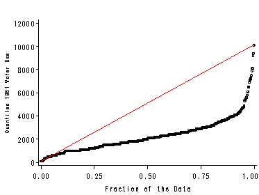
Figure 1.5, page 12. SAS does not have a procedure or graph option for quantile plots. We will again show how to plot the graph manually here. A dataset sorted by water81 was created previously. We use it here to create a fraction variable.
data q81;
  set sorted81;

  obsid = _n_;
  fraction = (obsid - .5) / &n81;

  if obsid = 1 or obsid = &n81 then do;
    x = fraction;
    y = water81;
  end;
run;

axis1 order=(0 to 12000 by 2000)
      label=(angle=90 height=.75 'Quantiles 1981 Water Use');
axis2 order=(0 to 1 by .25)
      label=('Fraction of the Data');

symbol1 interpol=none value=circle color=black height=.5;
symbol2 interpol=join value=none color=red;

proc gplot data=q81;
  plot water81*fraction
  y*x / vaxis=axis1 vminor=0
        haxis=axis2 hminor=0
        noframe overlay;
run;
quit;
Quantile-Quantile Plots
Figure 1.7, page 14. SAS does not have a procedure or graph option to produce a Quantile-Quantile plot. Below we show you how to do this manually. Quantiles of 1980 water use:
proc sort data=in.concord1 out=sorted80;
  by water80;
run;
data qq1;
  merge sorted80(keep=water80)
        sorted81(keep=water81) /* created earlier*/
 /* could use either &n80 or &n81 here */
if _n_ = 1 then x = min(water80,water81);
if _n_ = 1 then x = min(water80,water81);
else if _n_ = &n81 then x = max(water80,water81);
y=x;
run;

axis1 order=(0 to 14000 by 2000) label=(angle=90 height=.75);
symbol1 interpol=none value=circle color=black height=.5;
symbol2 interpol=join value=none color=red;

proc gplot data=qq1;
  plot water81*water80  y*x / vminor=1 vaxis=axis1 hminor=1
			      noframe overlay;
run;
quit;
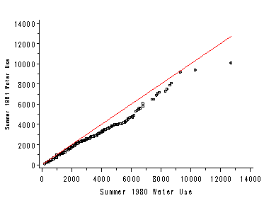
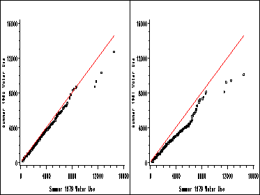
Figure 1.8, page 14. The two plots in this figure are first graphed separately and output to a graphics catalog. Then they are graphed together using proc greplay. The variable water79 has missing values. Records with missing values on either the horizontal or vertical axis must be excluded. Otherwise, the quantiles will mis-merge in a later data step. Quantiles of 1979 water use:
proc sort data=in.concord1 out=dat79(keep=water79);
  where water79^=.;
  by water79;
run;
Quantiles of 1980 water use:
proc sort data=in.concord1 out=dat80(keep=water80);
  where water79^=.;
  by water80;
run;
Quantiles of 1981 water use:
proc sort data=in.concord1 out=dat81(keep=water81);
  where water79^=.;
  by water81;
run;
Merge the quantiles one-to-one and define two (x80,y80) points and two (x81,y81) points for the reference lines.
data qq2;
  merge dat79 dat80 dat81; /* 1-1 merge */

  if _n_ = 1 then do;
    x80 = min(water79,water80);
    x81 = min(water79,water81);
  end;
  else if _n_ = &n79 then do;
    x80 = max(water79,water80);
    x81 = max(water79,water81);
  end;

  y80 = x80;
  y81 = x81;
run;
Delete the contents of the graphics catalog named mycat. Otherwise, you’ll have to keep track of how the graphs are named. Don’t worry if you get an error message that memname mycat is unknown.
proc greplay igout=mycat tc=tempcat nofs;
  delete _all_;
run;
Plot left graph and output to mycat.
axis1 order=(0 to 16000 by 4000)
      label=(angle=90 color=black height=0.75);
axis2 order=(0 to 16000 by 4000)
      label=(angle=0 color=black);

symbol1 color=black interpol=none value=circle height=0.5;
symbol2 color=red interpol=join value=none;

proc gplot data=qq2 gout=mycat;
  plot water80*water79
       y80*x80 / vminor=3 vaxis=axis1
                 hminor=3 haxis=axis2
                 noframe overlay;
run;
quit;
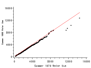
Right graph (uses same axis and symbols as left graph).
proc gplot data=qq2 gout=mycat;
  plot water81*water79
       y81*x81 / vminor=3 vaxis=axis1
                 hminor=3 haxis=axis2
                 noframe overlay;
run;
quit;
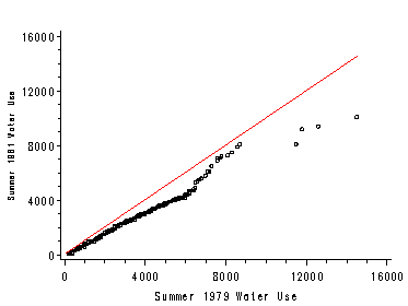
Replay the left and right graphs on one figure using SAS’ h2 template.
proc greplay nofs igout=mycat tc=sashelp.templt template=h2;
  treplay 1:gplot 2:gplot1;
run;
Quantile Normal Plots
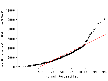
Figure 1.9, page 16.
proc univariate data=in.concord1 noprint;
  var water81;
  probplot / normal(mu=est sigma=est color=red) noframe;
run;
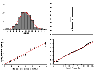
Selecting an Appropriate Power
Figure 1.13, page 20.
We have skipped this example.
The natural log of water81 is not a variable in the concord1 dataset. So first create the variable using the log function.
data c2;
  set sorted81;
  ln81 = log(water81);
  label ln81='Natural Log of Water Use';
run;
data c3;
  set c2;

  wat81_03 = water81**0.3;
  cvar=0;
run;
Step 2. Turn off the graphics display and clear mycat.
goptions nodisplay;
proc greplay igout=mycat tc=tempcat nofs;
  delete _all_;
run;
Step 3. Plot each graph individually and output to mycat. Top-left Histogram:
proc univariate data=c3 gout=mycat noprint;
  var wat81_03;
  histogram / normal(color=red)
              cfill=grey
              noframe
              vaxis=(0 to 30 by 10);
run;
Bottom-left Symmetry Plot: We have removed this example.
Top-right Boxplot:
axis2 label=none value=none major=none minor=none;

proc boxplot data=c3 gout=mycat;
  plot wat81_03*cvar / cboxes=black
                       noframe
                       boxstyle=schematic
                       haxis=axis2
                       vaxis=(2 to 18 by 2);
run;
Bottom-right Quantile Normal Plot:
proc univariate data=c3 noprint gout=mycat;
  var wat81_03;
  probplot / normal(mu=est sigma=est color=red) noframe;
run;
Step 4. Turn graphics display back on and replay the four graphs in mycat using SAS’ l2r2 template.
options display;
proc greplay nofs igout=mycat tc=sashelp.templt template=l2r2;
treplay 1:univar 2:gplot 3:boxplot 4:univar1 ;
run;
quit;