Survival Analysis by John P. Klein and Melvin L. Moeschberger Chapter 11: Regression Diagnostics | SAS Textbook Examples

Section 11.2: Cox-Snell Residuals for Assessing the Fit of a Cox Model

A data step creates a data set called bone_marrow1, and it can be downloaded here. We will use this dataset in this section.

data bone_marrow1;
   set bone_marrow;
  z1 = z1 -28;
  z2 = z2- 28;
  z1xz2 = z1 * z2;
  g1 = ( g = 1 );
  g2 = ( g = 2 );
  g3 = ( g = 3 );
  cons = 1;
  z7c = z7 / 30 - 9;
run;

Fig. 11.1 on page 330.

proc phreg data = bone_marrow1;
  model t2*dfree(0) = z1 z2 z1xz2 g2 g3 z7c z8 z10 ;
  output out = figure11_1 LOGSURV = h /method = ch;  /*-logsurv is the cox-snell residual*/
run;

data figure11_1a;
  set figure11_1;
  h = -h;
  cons = 1;
run;
proc phreg data = figure11_1a ;
  model  h*dfree(0) = cons;
  output out = figure11_1b logsurv = ls /method = ch;
run;
data figure11_1c;
  set figure11_1b;
    haz = - ls;
run;
proc sort data = figure11_1c;
 by h;
run;
title "Figure 11.1";
axis1 order = (0 to 3 by .5) minor = none;
axis2 order = (0 to 3 by .5) minor = none label = ( a=90);
symbol1 i = stepjl c= blue;
symbol2 i = join c = red l = 3;
proc gplot data = figure11_1c;
  plot haz*h =1 h*h =2 /overlay haxis=axis1 vaxis= axis2;
  label haz = "Estimated Cumulative Hazard Rates";
  label h = "Residual";
run;
quit;

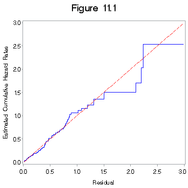
Figure 11.2 on page 331.

proc sort data = figure11_1a;
  by z10;
run;
proc phreg data = figure11_1a ;
  model  h*dfree(0) = cons;
  output out = fill_2b logsurv = ls /method = ch;
  by z10;
run;
data fill_2b1;
  set fill_2b;
  if z10 = 0 then haz1 = -ls;
  if z10 = 1 then haz2 = -ls;
run;
proc sort data = fill_2b1;
  by h;
run;
title "Figure 11.2";
symbol1 i = stepjl c= blue;
symbol2 i = stepjl c = red l = 3;
symbol3 i = join c = black;

proc gplot data = fill_2b1;
  plot haz1*h = 1 haz2*h = 2 h*h=3 /overlay haxis=axis1 vaxis=axis2 ;
  label haz1 = "Log Cumulative Hazard Rate";
  label h= "Residual";
run;
quit;

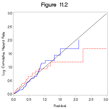
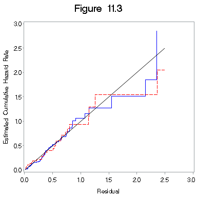
Figure 11.3 on page 332.

proc phreg data = bone_marrow1 ;
  model  t2*dfree(0) =  z1 z2 z1xz2 g2 g3 z7 z8 ;
  strata z10;
  output out = figure11_3 logsurv = h /method=ch;
run;
data figure11_3a;
  set figure11_3;
    cons = 1;
	h = -h;
run;
proc sort data = figure11_3a;
 by z10;
run;
proc phreg data = figure11_3a ;
  model  h*dfree(0) = cons;
  output out = fig11_t logsurv = ls /method = ch;
  by z10;
run;
data fig11_t;
  set fig11_t;
    if z10 = 0 then haz1 = - ls;
	if z10 = 1 then haz2 = - ls;
run;
proc sort data = fig11_t;
 by h;
run;
options label;

title "Figure 11.3";
axis1 order = (0 to 3 by .5) minor = none;
axis2 order = (0 to 3 by .5) minor = none label = ( a=90);
symbol1 i = stepjl c= blue;
symbol2 i = stepjl c = red l = 3;
symbol3 i = join c = black;

proc gplot data = fig11_t;
  plot haz1*h = 1 haz2*h = 2 h*h=3 /overlay haxis=axis1 vaxis=axis2 ;
  label haz1 = "Estimated Cumulative Hazard Rate";
  label h= "Residual";
run;
quit;

Section 11.3: Determining the Functional Form of a Covariate: Martingale Residuals

data sec1_10;
input type dtype time ind kscore wtime;
cards;
1 1 28 1 90 24
1 1 32 1 30 7
1 1 49 1 40 8
1 1 84 1 60 10
1 1 357 1 70 42
1 1 933 0 90 9
1 1 1078 0 100 16
1 1 1183 0 90 16
1 1 1560 0 80 20
1 1 2114 0 80 27
1 1 2144 0 90 5
1 2 2 1 20 34
1 2 4 1 50 28
1 2 72 1 80 59
1 2 77 1 60 102
1 2 79 1 70 71
2 1 42 1 80 19
2 1 53 1 90 17
2 1 57 1 30 9
2 1 63 1 60 13
2 1 81 1 50 12
2 1 140 1 100 11
2 1 81 1 50 12
2 1 252 1 90 21
2 1 524 1 90 39
2 1 210 0 90 16
2 1 476 0 90 24
2 1 1037 0 90 84
2 2 30 1 90 73
2 2 36 1 80 61
2 2 41 1 70 34
2 2 52 1 60 18
2 2 62 1 90 40
2 2 108 1 70 65
2 2 132 1 60 17
2 2 180 0 100 61
2 2 307 0 100 24
2 2 406 0 100 48
2 2 446 0 100 52
2 2 484 0 90 84
2 2 748 0 90 171
2 2 1290 0 90 20
2 2 1345 0 80 98
;
run;

proc phreg data = sec1_10;
  model time*ind(0) = wtime dtype type kscore;
  output out = figure11_4 RESMART = mgale ;
run;
proc loess data=figure11_4;
  ods output OutputStatistics=figure11_4a;
  model mgale = wtime / smooth=0.6 direct;
run;
quit;
proc sort data = figure11_4a;
  by wtime;
run;
axis1 order = (-2.0 to 1 by .5) offset = (0, 2) label= (a = 90) minor = none;
axis2 order = (0 to 200 by 50) minor = none;
symbol1 i = none v = dot h = 1.5 c = blue;
symbol2 i = join v = none c = red;
title "Figure 11.4";
proc gplot data = figure11_4a;
  format depvar f4.1;
  format wtime f4.1;
  plot depvar*wtime = 1 pred*wtime = 2 /haxis = axis2 vaxis = axis1 overlay;
  label depvar = "Martingle Residual";
  label wtime = "Waiting Time to Transplant (months)";
run;
quit;

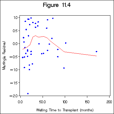
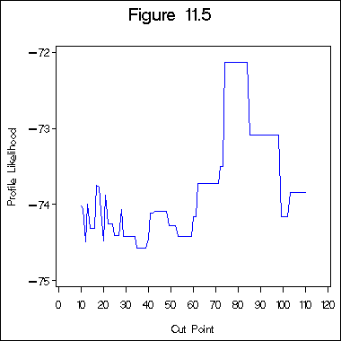
Figure 11.5 on page 336.

%macro profile(data, dep, indep, step);
  
  ods listing close;
  proc sql;
  drop table _profile_;
  quit;
  proc sql;
  create table _profile_ (type = data ,
                          logr char(12),
		          step char(12));
  quit;
  %do i = 10 %to 110 %by &step;
  data _temp_;
    set &data;
	  if wtime < &i then z2 = 0;
	  else z2 = 1;
  run;
  proc phreg data = _temp_ ;
     model &dep = &indep z2;
     ods output FitStatistics = _ll_;
  run;
  data _null_;
    set _ll_;
	if _n_ = 1 then
	call symput('logr', withcovariates);
  run;
  proc sql;
    insert into _profile_
	   values("&logr", "&i");
    quit;
%end;
  data _profile_;
    set _profile_;
	logr1 = - input(logr, 8.)/2;
	step1 = input(step, 8.);
  run;

  ods listing;
  proc gplot data = _profile_;
    title "Figure 11.5";
    symbol i = join c = blue ;
    axis1 minor = none label = (a=90);
    axis2 minor = none order = (0 to 120 by 10);
    format logr1 3.0;
    format step1 4.0;
    plot logr1*step1 = 1 /haxis = axis2 vaxis = axis1;
    label logr1 = "Profile Likelihood";
    label step1 = "Cut Point";
  run;
  quit;
%mend;
%profile(figure11_4, time*ind(0), dtype type kscore, 1);

Section 11.4: Graphical Checks of the Proportional Hazards Assumption

Figure 11.6 on page 339.

data sec1_9;
  input time type ind;
cards;
0.030 1 1
0.493 1 1
0.855 1 1
1.184 1 1
1.283 1 1
1.480 1 1
1.776 1 1
2.138 1 1
2.500 1 1
2.763 1 1
2.993 1 1
3.224 1 1
3.421 1 1
4.178 1 1
4.441 1 0
5.691 1 1
5.855 1 0
6.941 1 0
6.941 1 1
7.993 1 0
8.882 1 1
8.882 1 1
9.145 1 0
11.480 1 1
11.513 1 1
12.105 1 0
12.796 1 1
12.993 1 0
13.849 1 0
16.612 1 0
17.138 1 0
20.066 1 1
20.329 1 0
22.368 1 0
26.776 1 0
28.717 1 0
28.717 1 0
32.928 1 0
33.783 1 0
34.221 1 0
34.770 1 0
39.593 1 0
41.118 1 0
45.003 1 0
46.053 1 0
46.941 1 0
48.289 1 0
57.401 1 0
58.322 1 0
60.625 1 0
0.658 2 1
0.822 2 1
1.414 2 1
2.500 2 1
3.322 2 1
3.816 2 1
4.737 2 1
4.836 2 0
4.934 2 1
5.033 2 1
5.757 2 1
5.855 2 1
5.987 2 1
6.151 2 1
6.217 2 1
6.447 2 0
8.651 2 1
8.711 2 1
9.441 2 0
10.329 2 1
11.480 2 1
12.007 2 1
12.007 2 0
12.237 2 1
12.401 2 0
13.059 2 0
14.474 2 0
15.000 2 0
15.461 2 1
15.757 2 1
16.480 2 1
16.711 2 1
17.204 2 0
17.237 2 1
17.303 2 0
17.664 2 0
18.092 2 1
18.092 2 0
18.750 2 0
20.625 2 0
23.158 2 1
27.730 2 0
31.184 2 0
32.434 2 0
35.921 2 0
42.237 2 0
44.638 2 0
46.480 2 0
47.467 2 0
48.322 2 0
56.086 2 1
;
end;
data sec1_9a;
  set sec1_9;
  cons = 1;
  type1 = type - 1;
run;
proc phreg data = sec1_9a ;
  model  time*ind(0) = cons;
  strata type1;
  output out = figure11_6 logsurv = ls /method = ch;
run;
data figure11_6a;
  set figure11_6 ;
    logh = log (-ls);
	if type1 = 0 then logh1 = logh;
	if type1 = 1 then logh2 = logh;
run;
proc sort data = figure11_6a;
 by time;
run;
options label;
goptions reset = all;
title "Figure 11.6";
axis1 order = (0 to 25 by 5) minor = none;
axis2 order = (-4 to 0 by 1) minor = none label = ( a=90);
symbol1 i = stepjl c= blue;
symbol2 i = stepjl c = red l = 3;

proc gplot data = figure11_6a;
  plot logh1*time = 1 logh2*time = 2 /overlay haxis=axis1 vaxis=axis2 ;
  label logh1 = "Log Cumulative Hazard Rate";
  label time= "Time on Study";
run;
quit;

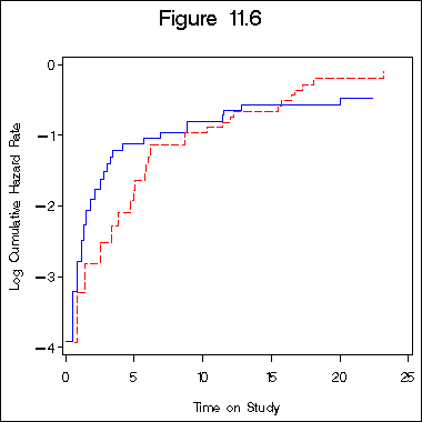
Figure 11.7 on page 340.

data figure11_6b;
  set figure11_6a;
   retain l1 l2 -5;
   if logh1 ~= . then l1 = logh1;
   if logh2 ~= . then l2 = logh2;
   diff = l2 - l1;
run;
goptions reset = all;
goptions  ftext = swiss htitle = 5 htext = 3 gunit = pct 
	border cback = white hsize = 4in vsize = 4in;
	filename outgraph 'e:survival_analysissashttps://stats.idre.ucla.edu/wp-content/uploads/2016/02/ch11_7.gif';
	goptions gsfname = outgraph dev = gif570; 

axis1 order = (0 to 25 by 5) minor = none;
axis2 order = (-1.5  to 1 by .5) minor = none label = ( a=90);
symbol1 i = stepjl c= blue;
title "Figure 11.7";
proc gplot data = figure11_6b;
  plot diff*time /haxis= axis1 vaxis=axis2 vref=0;
  label diff = "Difference in Cumulative Hazard Rates";
  label time = "Time on Study";
run;
quit;

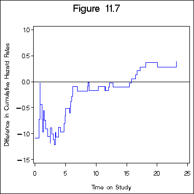
Figure 11.8 on page 341.

data figure11_6c;
  set figure11_6b;
  retain h1 h2 0;
  if type1 = 0 then h1 = -ls;
  if type1 = 1 then h2 = -ls;
run;
proc sort data = figure11_6c;
  by l1;
run;

symbol1 c = blue i = stepjl;
symbol2 c = black i = join;
title "Figure 11.8";
axis1 order = (0 to 1 by .2) minor = none;
axis2 order = (0  to 1 by .2) minor = none label = ( a=90); 
proc gplot data = figure11_6c;
  plot h2*h1 = 1 h1*h1=2 /overlay haxis = axis1 vaxis = axis2;
  label h2 = "Auto";
  label h1 = "Allo";
run;
quit;

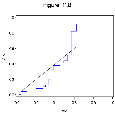
Figure 11.9 on page 342.

proc phreg data = bone_marrow1 ;
  model  t2*dfree(0) = cons;
  strata z10;
  output out = figure11_9 logsurv = ls /method = ch;
run;
data figure11_9a;
  set figure11_9 ;
    logh = log (-ls);
	if z10 = 0 then logh1 = logh;
	if z10 = 1 then logh2 = logh;
run;
proc sort data = figure11_9a;
 by t2;
run;

title "Figure 11.9";
axis1 order = (0 to 1200 by 200) minor = none;
axis2 order = (-4 to 0 by 1) minor = none label = ( a=90);
symbol1 i = stepjl c= blue;
symbol2 i = stepjl c = red l = 3;

proc gplot data = figure11_9a;
  plot logh1*t2 = 1 logh2*t2 = 2 /overlay haxis=axis1 vaxis=axis2 ;
  label logh1 = "Log Cumulative Hazard Rate";
  label t2= "Time on Study";
run;
quit;

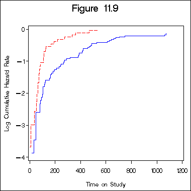
Figure 11.10 on page 343.

data figure11_9b;
  set figure11_9a;
   retain l1 l2 -5;
   if logh1 ~= . then l1 = logh1;
   if logh2 ~= . then l2 = logh2;
   diff = l2 - l1;
run;

axis1 order = (0 to 1200 by 200) minor = none;
axis2 order = (0  to 1.6 by .4) minor = none label = ( a=90);
symbol1 i = stepjl c= blue;
title "Figure 11.10";
proc gplot data = figure11_9b;
  plot diff*t2 /haxis= axis1 vaxis=axis2;
  label diff = "Difference in Cumulative Hazard Rates";
  label t2 = "Time on Study";
run;
quit;

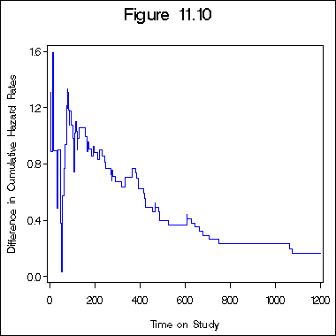
Figure 11.11 on page 344.

data figure11_11;
  set figure11_9b;
  retain h1 h2 0;
  if z10 = 0 then h1 = -ls;
  if z10 = 1 then h2 = -ls;
run;
proc sort data = figure11_11;
  by l1;
run;

symbol1 c = blue i = stepjl;
symbol2 c = black i = join;
title "Figure 11.11";
axis1 order = (0 to 1 by .2) minor = none;
axis2 order = (0  to 1 by .2) minor = none label = ( a=90); 
proc gplot data = figure11_11;
  plot h2*h1 = 1 h1*h1=2 /overlay haxis = axis1 vaxis = axis2;
  label h2 = "MTX Group";
  label h1 = "No MTX Group";
run;
quit;

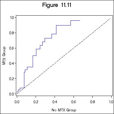
Figure 11.12 on page 345.

data bone_z7cat;
  set bone_marrow1;
  if z7c <= -5 then cz7 = 0;
  if -5 < z7c <= -3.06 then cz7 = 1;
  if -3.06 < z7c <= 0 then cz7 = 2;
  if 0 < z7c then cz7 = 3;
run;
proc phreg data = bone_z7cat;
  model t2*dfree(0) = z1 z2 z1xz2 g2 g3 z8 z10 ;
  strata cz7;
   baseline out = figure11_12 LOGSURV = h ;
run;
data figure11_12a;
  set figure11_12;
  if h ~= 0 then lgh = log(-h);
run;
proc sort data = figure11_12a;
 by t2;
run;

title "Figure 11.12";
axis1 order = (0 to 1200 by 200) offset = (5,2) minor = none;
axis2 order = (-4.5 to .5 by 1) offset = (5,5) minor = none label = ( a=90);
symbol1 i = stepjl c= blue;
symbol2 i = stepjl c = red l = 3;
symbol3 i = stepjl c = green l = 2;
symbol4 i = stepjl c = black l = 20;
legend label=none value=(h=2 font=swiss '<=-5' '-5, -3.06' '-3.06, 0' '>0')
       position=(bottom right inside) mode=share cborder=black;

proc gplot data = figure11_12a;
  plot lgh*t2 = cz7 /legend=legend haxis=axis1 vaxis=axis2 ;
  label lgh = "Log Cumulative Hazard Rate";
  label t2= "Time on Study";
run;
quit;

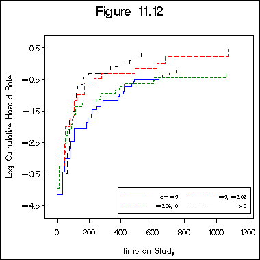
Figure 11.13 on page 346.

proc sort data = figure11_12;
by t2;
proc transpose data = figure11_12 out = fig11_13(keep = t2 group0-group3) prefix=group;
by t2;
id cz7;
var h ;
run;
proc print data=fig11_13;
run;
data fig11_13a;
  set fig11_13;
  retain lgh1 lgh2  lgh3 lgh4 0;
  if group0 ~= . then lgh1 = log(-group0);
  if group1 ~= . then lgh2 = log(-group1);
  if group2 ~= . then lgh3 = log(-group2);
  if group3 ~= . then lgh4 = log(-group3);
   diff2 = lgh2 - lgh1;
   diff3 = lgh3 - lgh1;
   diff4 = lgh4 - lgh1;
run;

axis1 order = (0 to 1200 by 200) minor = none;
axis2 order = (-1  to 2 by .5) minor = none label = ( a=90);
symbol1 i = stepjl c= black;
symbol2 i = stepjl c = red l = 3;
symbol3 i = stepjl c = green l = 2;
legend label=none value=(h=2 font=swiss '2 vs. 1' '3 vs. 1' '4 vs. 1')
       position=(bottom right inside) mode=share cborder=black;
title "Figure 11.13";
proc gplot data = fig11_13a;
  plot diff2*t2 = 1 diff3*t2 = 2 diff4*t2 = 3 / legend = legend overlay haxis= axis1 vaxis=axis2;
  label diff2 = "Difference in Cumulative Hazard Rates";
  label t2 = "Time on Study";
run;
quit;

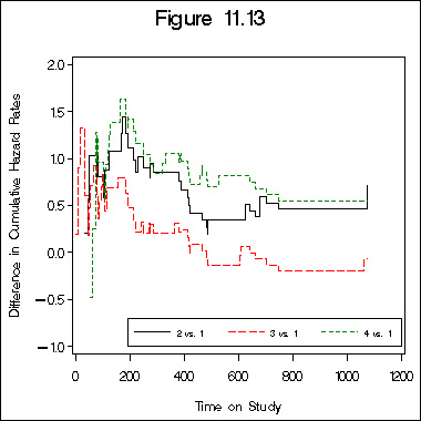
Figure 11.14 on page 347.

data fig11_14;
  set fig11_13;
  retain h1 h2 h3 h4 0;
  if group0 ~= . then h1 = -group0;
  if group1 ~= . then h2 = -group1;
  if group2 ~= . then h3 = -group2;
  if group3 ~= . then h4 = -group3;
run;
proc sort data = fig11_14;
  by h1;
run;

symbol1 i = stepjl c= black;
symbol2 i = stepjl c = red l = 3;
symbol3 i = stepjl c = green l = 2;
title "Figure 11.14";
axis1 order = (0 to .8 by .2) minor = none;
axis2 order = (0  to 1.4 by .2) minor = none label = ( a=90); 
legend label=none value=(h=2 font=swiss 'Strata 2' 'Strata 3' 'Strata 4')
       position=(bottom right inside) mode=share cborder=black;
proc gplot data = fig11_14;
  plot h2*h1 = 1 h3*h1 = 2 h4*h1 = 3 /legend = legend overlay haxis = axis1 vaxis = axis2;
  label h2 = "Estimated Cumulative Hazard Rate for jth Strata";
  label h1 = "Estimated Cumulative Hazard Rate for Strata with centered Waiting Time <=-5";
run;
quit;

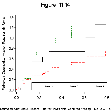
Figure 11.15 on page 348.

data sec1_9a;
  set sec1_9;
  cons = 1;
run;
proc phreg data = sec1_9a ;
  model time*ind(0)=cons ;
  output out = try15 logsurv=h;
run;
proc sql noprint;
  select count(time) into :t1-:t2
  from sec1_9a
  group by type;
quit;
proc sort data = sec1_9;
by time ind;
proc sort data = try15;
by time ind;
data try15a;
  merge sec1_9 try15;
   by time;
   retain n1 n2 h1 h2 c1 c2 0;
   if h ~=. then do;
   if type = 1 then do ;
     c1 = c1 + 1;
     n1 = n1 + ind;
	 h1 = -h + h1;
	 end;
   else if type = 2 then do;
     c2 = c2 + 1;
     n2 = n2 + ind;
	 h2 = -h + h2;
	 end; 
     end;
	 hh1 = h1 - h*(&t1-c1);
	 hh2 = h2 - h*(&t2-c2);
run;

axis1 order = (0 to 30 by 5) label=('Number of Failures') minor=none;
axis2 order = (0 to 30 by 5) label=(a=90 'Estimated Cumulative Hazard Rates') minor=none;
symbol1 i = join c = red ;
symbol2 i = join c = blue;
symbol3 i = join c = black;
title 'Figure 11.15';
proc gplot data = try15a;
plot hh1*n1 hh2*n2 n1*n1 /overlay haxis = axis1 vaxis = axis2;
run;
quit;

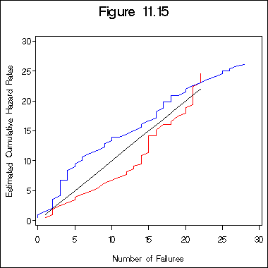
Figure 11.16 on page 349.

proc phreg data = bone_marrow1;
    model t2*dfree(0) = z1 z2 z1xz2 g2 g3 z7;
    baseline out = fig11_16 LOGSURV = h ;
run;
proc sql noprint;
  select count(t2) into :t1-:t2
  from  bone_marrow1
  group by z10;
quit;
proc sort data = bone_marrow1;
by t2;
data try16a;
  merge bone_marrow1 fig11_16 ;
   by t2;
   retain n1 n2 c1 c2 h1 h2 0;
   if h ~=. then do;
   if z10 = 0  then do ;
     c1 = c1 + 1;
     n1 = n1 + dfree;
	 h1 = h1 - h;
	 end;
   if z10 = 1 then do;
     c2 = c2 + 1;
     n2 = n2 + dfree;
	 h2 = h2 - h;
	 end;
	 end;
	 hh1 = h1 - h*(&t1-c1);
	 hh2 = h2 - h*(&t2-c2);
run;

axis1 order = (0 to 60 by 10) minor = none label=('Number of Failures');
axis2 order = (0 to 60 by 20) minor = none label=(a=90 'Estimated Cumulative Hazard Rates');
symbol1 i = join c = red ;
symbol2 i = join c = blue;
symbol3 i = join c = black;
title 'Figure 11.16';
proc gplot data = try16a;
plot hh1*n1 hh2*n2 n1*n1 /overlay haxis = axis1 vaxis = axis2;
run;
quit;

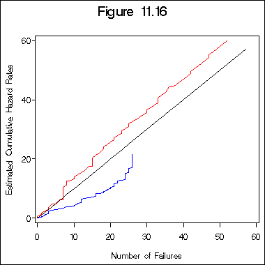
Figure 11.17 is omitted here.

Figure 11.18 on page 352.

Section 11.5: Deviance Residuals

Section 11.6: Checking the Influence of Individual Observations

Section 11.7: Assessing the Fit of the Additive Model