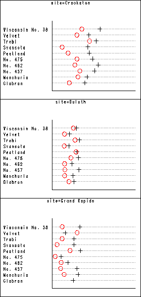
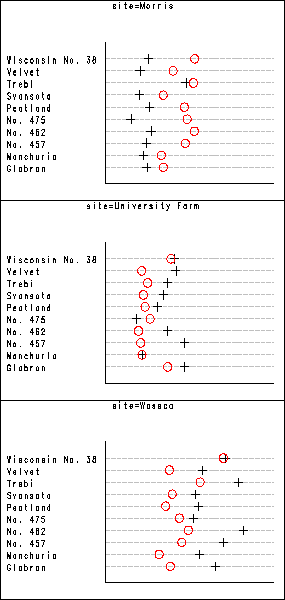
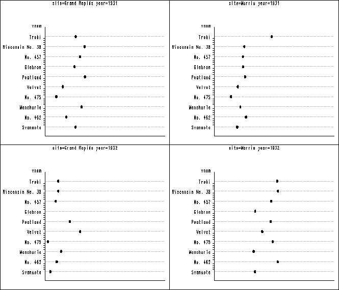
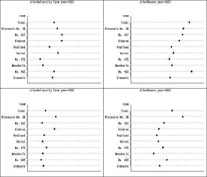
Figure 1.1 on page 4 using barley data set. Using the by statement in proc gplot, SAS automatically creates all the subplots. We then use proc greplay to put them all together in one plot.
proc sort data = clev1.barley out = barley;
  by site;
run;
goptions reset = all vsize=1.6 hsize= 2.5 htext=.5;
symbol1 v = plus c = black;
symbol2 v = circle c = red;
axis1 order = (15 to 75 by 15) value=none major = none
				minor = none label=('')
axis2 label = ('') offset=(1,1) major=none;
proc gplot data = barley;
  by site;
  plot variety*yield=year / nolegend haxis=axis1 vaxis= axis2
	                    cvref= ligr lvref = 3 autovref noframe;
 run;
quit;
We put three of them together to make one single plot. So we end up with two plots instead of one. They look better in two plots as in one single plot. One can use the same procedure shown below to put the two plots together again to form a single one. But one has to be careful about the ratio of the plots.
goptions vsize = 0 vpos=0 display hsize=0;
proc greplay igout=work.gseg tc=sashelp.templt
             template=v3 nofs;
   treplay 1:gplot 2:gplot1 3: gplot2;
   treplay 1:gplot3 2:gplot4 3:gplot5;
run;
quit;
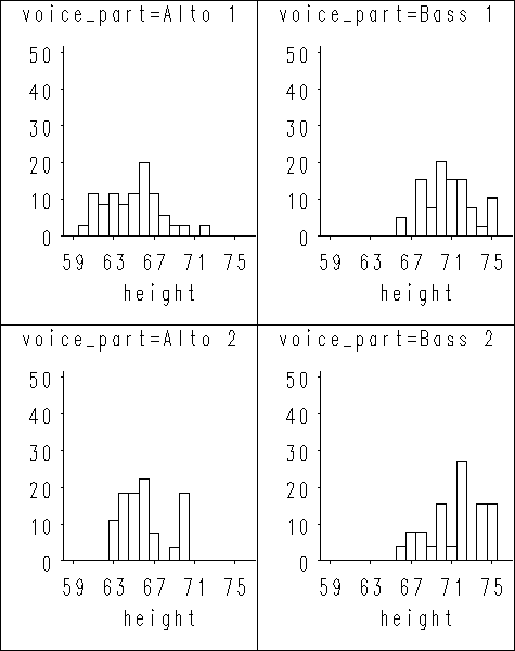
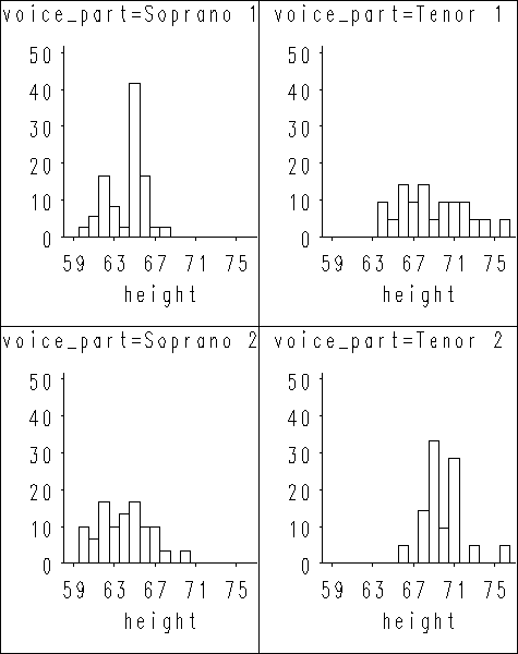
Figure 1.2 on page 7 using singer data set. We first sort the data set by variable voice_part so we can make use of the by statement in proc univariate. After proc univariate produces all the plots, we put them together as two plots using proc greplay.
proc sort data = singer;
  by voice_part ;
run;

proc greplay nofs igout = work.gseg;
 delete _all_;
run;

goptions reset = all vsize=2 hsize= 2;
proc univariate data = singer noprint;
  by voice_part ;
  histogram height /vaxis=0 10 20 30 40 50 vaxislabel=''
midpoints=(59 to 76 by 1) noframe;
  label height = '';
run;

goptions vsize = 0 vpos=0 display hsize=0;
proc greplay igout= work.gseg tc=sashelp.templt
             template=l2r2 nofs;
   treplay 1:univar 2:univar1 3: univar2 4: univar3;
   treplay 1:univar4 2:univar5 3:univar6 4: univar7;
run;
quit;
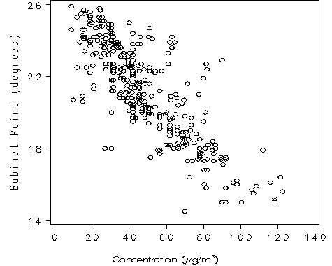
Figure 1.3 on page 9. It is a simple gplot procedure to produce the scatter plot. We used the footnote statement with the move option to get Greek letter and superscript in the title.
goptions reset = all vsize=4 hsize= 4;
symbol v=circle c=black ;
axis1 order = (0 to 140 by 20) minor = none label=('');
axis2 order = (14 to 26 by 4) minor = none label=(a=90 'Babinet Point (degrees)');
footnote f = swiss h = 1 'Concentration ('
	 f =greek 'm' f = swiss 'g/m' move=(+0, +0.5) h= .5 '3' move=(-0, -0.5) h=1 ')';
proc gplot data = clev1.polarization;
  plot babinet*concentration /haxis=axis1 vaxis=axis2;
run;
quit;
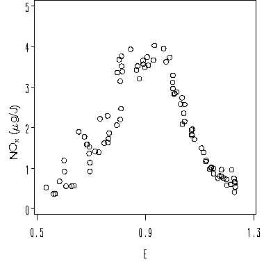
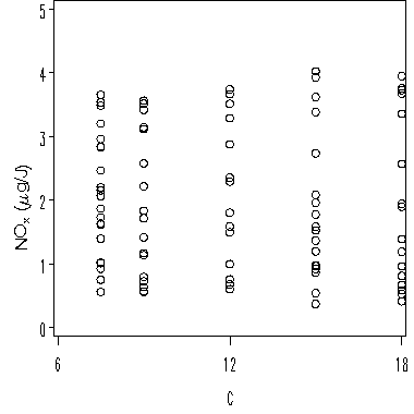
Figure 1.4 and Figure 1.5 on page 11.
goptions reset = all vsize=4 hsize= 4;
symbol v = circle c=black h=0.8;
axis1 order = (.5 to 1.3 by .4) minor = none label = ('E');
axis2 order = (0 to 5 by 1) minor = none label=('');
title angle=90 h = 1 'NO' move=(+0.5, -0) h=.6 'x '
	  move=(-.5, +0) h = 1 '(' font = greek 'm' font = swiss 'g/J)';
proc gplot data = clev1.ethanol;
  plot nox*e /haxis=axis1 vaxis=axis2;
run;
quit;
goptions reset = all vsize=4 hsize= 4;
symbol v = circle c=black h=0.8;
axis1 order = (6 to 18 by 6) minor = none label = ('C');
axis2 order = (0 to 5 by 1) minor = none label=('');
title angle=90 h = 1 'NO' move=(+0.5, -0) h=.6 'x '
	  move=(-.5, +0) h = 1 '(' font = greek 'm' font = swiss 'g/J)';
proc gplot data = clev1.ethanol;
  plot nox*c /haxis=axis1 vaxis=axis2;
run;
quit;
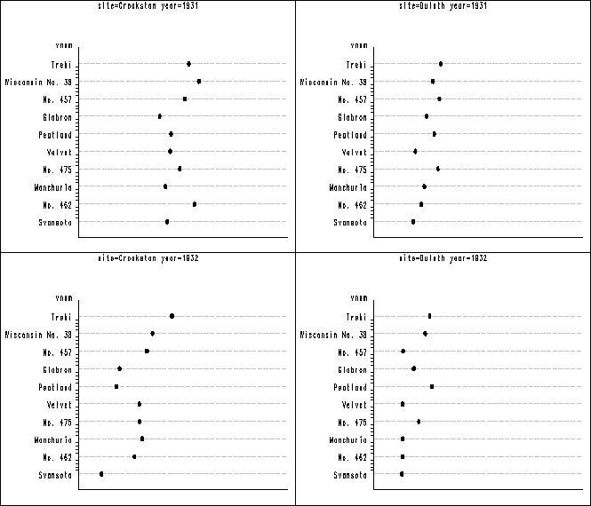
Figure 1.6 on page 13. In figure 1.1 above the vertical axis has different order from the plot in the book. In order to get them to be in the same order, we have to recode the variable shown below. Then we have to label the vertical axis using the value option to specify what should be for each of the tick on the axis. After all the plots are created, we again use proc greplay to group the plots together into three panels. Notice that the orders of the plots are different from the book, but each individual plot is the same.
data barley;
  set clev1.barley;
  if variety = 'Trebi' then vnum = 10;
  if variety = 'Wisconsin No. 38' then vnum = 9;
  if variety = 'No. 457' then vnum = 8;
  if variety = 'Glabron' then vnum = 7;
  if variety = 'Peatland' then vnum = 6;
  if variety = 'Velvet' then vnum = 5;
  if variety = 'No. 475' then vnum = 4;
  if variety = 'Manchuria' then vnum = 3;
  if variety = 'No. 462' then vnum = 2;
  if variety = 'Svansota' then vnum = 1;
run;
proc sort data = barley ;
  by site year;
run;
proc greplay nofs igout = work.gseg;
 delete _all_;
run;
goptions reset = all vsize=2 hsize= 3.5 htext=.5;
symbol2 v = dot c = black h = .5;
axis1 order = (15 to 75 by 15) value=none major = none
				minor = none label=('');
axis2 value = (tick = 1 'Svansota' tick = 2 'No. 462' tick = 3 'Manchuria'
      tick = 4 'No. 475' tick = 5 'Velvet' tick = 6 'Peatland' tick = 7 'Glabron'
      tick = 8 'No. 457' tick = 9 'Wisconsin No. 38' tick = 10 'Trebi')
      offset=(1,1) major=none;
proc gplot data = barley;
  by site year;
  plot vnum*yield / nolegend haxis=axis1 vaxis= axis2
	            cvref= ligr lvref = 3 autovref noframe;
 run;
quit;
goptions vsize = 0 vpos=0 display hsize=0;
proc greplay igout=work.gseg tc=sashelp.templt
             template=l2r2 nofs;
   treplay 1:gplot 2:gplot1 3: gplot2 4: gplot3;
   treplay 1:gplot4 2:gplot5 3:gplot6 4: gplot7;
   treplay 1:gplot8 2:gplot9 3:gplot10 4: gplot11;
run;
quit;

