It is possible to estimate recursive path models using ordinary least squares regression, but using the SAS proc calis can make the processes easier and will also provide estimates of direct and indirect effects.
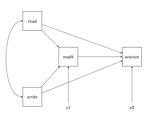
Let’s say that we want to estimate the following path model using the hsb2 (hsb2.sas7bdat) dataset.
We will begin computing the correlation between the two exogenous variables, read and write. We assume that the data file, hsb2.sas7bdat, is located in the data directory on the C: drive. You may need to change these values for your particular computer configuration.
proc corr data='C:datahsb2';
  var read write;
run;


The CORR Procedure

2 Variables: READ WRITE


Simple Statistics

Variable  N    Mean      Std Dev    Sum     Minimum    Maximum  Label
READ     200  52.23000  10.25294   10446   28.00000   76.00000   reading score
WRITE    200  52.77500   9.47859   10555   31.00000   67.00000   writing score


Pearson Correlation Coefficients, N = 200
Prob > |r| under H0: Rho=0

                    READ          WRITE

READ              1.00000       0.59678
reading score                    <.0001

WRITE             0.59678       1.00000
writing score      <.0001
This path analysis is really just two regression models. The first model is math = constant + read + write while the second model is science = constant + math + read + write. In proc calis we set up the model by entering the response variable with each predictor. In the effpart part of the command we list the paths for direct and indirect effects.
proc calis data='C:datahsb2';
  path                      /* specification of path model */
   science <- math ,
   science <- read ,
   science <- write,
   math    <- read ,
   math    <- write;
  effpart                   /* for direct and indirect effects */
   science <- read write;
run;
We can now run the proc calis command which produces the output shown below. There is a lot of output but we will be focusing on the standardized results given near the end and shown in bold.
The CALIS Procedure
Covariance Structure Analysis: Model and Initial Values

     Modeling Information

Data Set            WC000001.HSB2
N Records Read      200
N Records Used      200
N Obs               200
Model Type          PATH
Analysis            Covariances


       Variables in the Model

Endogenous    Manifest    MATH  SCIENCE
             Latent
Exogenous     Manifest    READ  WRITE
             Latent

 Number of Endogenous Variables = 2
 Number of Exogenous Variables  = 2


         Initial Estimates for PATH List

----------Path----------    Parameter      Estimate

SCIENCE    <---    MATH     _Parm1                .
SCIENCE    <---    READ     _Parm2                .
SCIENCE    <---    WRITE    _Parm3                .
MATH       <---    READ     _Parm4                .
MATH       <---    WRITE    _Parm5                .


  Initial Estimates for Variance Parameters

Variance
Type         Variable    Parameter      Estimate

Exogenous    READ        _Add1                 .
             WRITE       _Add2                 .
Error        MATH        _Add3                 .
             SCIENCE     _Add4                 .
        WRITE    READ    _Add5                 .

NOTE: Parameters with prefix '_Add' are added by PROC CALIS.

                Simple Statistics

       Variable                  Mean       Std Dev

READ       reading score      52.23000      10.25294
WRITE      writing score      52.77500       9.47859
MATH       math score         52.64500       9.36845
SCIENCE    science score      51.85000       9.90089

The SAS System                                                   08:25
Thursday, May 12, 2011 180

The CALIS Procedure
Covariance Structure Analysis: Optimization

       Initial Estimation Methods

      1    Observed Moments of Variables
      2    McDonald Method
      3    Two-Stage Least Squares


             Optimization Start
             Parameter Estimates

   N    Parameter      Estimate      Gradient

   1    _Parm1          0.31901    -1.151E-16
   2    _Parm2          0.30153    1.8496E-16
   3    _Parm3          0.20653    -2.468E-32
   4    _Parm4          0.41695    -6.681E-16
   5    _Parm5          0.34112    2.5981E-31
   6    _Add1         105.12271     8.882E-34
   7    _Add2          89.84359    4.4965E-34
   8    _Add3          42.54028    6.5484E-18
   9    _Add4          49.01931    7.4888E-19
  10    _Add5          57.99673    6.3985E-34

       Value of Objective Function = 0


Levenberg-Marquardt Optimization

Scaling Update of More (1978)

Parameter Estimates                                10
Functions (Observations)                           10

                             Optimization Start

Active Constraints                     0    Objective Function               0
Max Abs Gradient Element    6.681129E-16    Radius                           1


                                     Optimization Results

Iterations                                    0  Function Calls
                       4
Jacobian Calls                                1  Active Constraints
                       0
Objective Function                            0  Max Abs Gradient
Element           6.681129E-16
Lambda                                        0  Actual Over Pred
Change                       0
Radius                                        1

Convergence criterion (ABSGCONV=0.00001) satisfied.
                          Fit Summary

Modeling Info        N Observations                             200
                    N Variables                                  4
                    N Moments                                   10
                    N Parameters                                10
                    N Active Constraints                         0
                    Baseline Model Function Value           1.8576
                    Baseline Model Chi-Square             369.6536
                    Baseline Model Chi-Square DF                 6
                    Pr > Baseline Model Chi-Square          <.0001
Absolute Index       Fit Function                            0.0000
                    Chi-Square                              0.0000
                    Chi-Square DF                                0
                    Pr > Chi-Square                              .
                    Z-Test of Wilson & Hilferty                  .
                    Hoelter Critical N                           .
                    Root Mean Square Residual (RMSR)        0.0000
                    Standardized RMSR (SRMSR)               0.0000
                    Goodness of Fit Index (GFI)             1.0000
Parsimony Index      Adjusted GFI (AGFI)                          .
                    Parsimonious GFI                        0.0000
                    RMSEA Estimate                               .
                    Probability of Close Fit                     .
                    ECVI Estimate                           0.1031
                    ECVI Lower 90% Confidence Limit              .
                    ECVI Upper 90% Confidence Limit              .
                    Akaike Information Criterion           20.0000
                    Bozdogan CAIC                          62.9832
                    Schwarz Bayesian Criterion             52.9832
                    McDonald Centrality                     1.0000
Incremental Index    Bentler Comparative Fit Index           1.0000
                    Bentler-Bonett NFI                      1.0000
                    Bentler-Bonett Non-normed Index              .
                    Bollen Normed Index Rho1                     .
                    Bollen Non-normed Index Delta2          1.0000
                    James et al. Parsimonious NFI           0.0000


                                  PATH List

                                                        Standard
----------Path----------    Parameter      Estimate         Error       t Value

SCIENCE    <---    MATH     _Parm1          0.31901       0.07610       4.19224
SCIENCE    <---    READ     _Parm2          0.30153       0.06816       4.42376
SCIENCE    <---    WRITE    _Parm3          0.20653       0.07023       2.94075
MATH       <---    READ     _Parm4          0.41695       0.05620       7.41912
MATH       <---    WRITE    _Parm5          0.34112       0.06079       5.61144


                           Variance Parameters

Variance                                              Standard
Type         Variable    Parameter      Estimate         Error       t Value

Exogenous    READ        _Add1         105.12271      10.53865       9.97497
             WRITE       _Add2          89.84359       9.00690       9.97497
Error        MATH        _Add3          42.54028       4.26470       9.97497
             SCIENCE     _Add4          49.01931       4.91423       9.97497


              Covariances Among Exogenous Variables

                                             Standard
Var1     Var2    Parameter      Estimate         Error       t Value

WRITE    READ    _Add5          57.99673       8.02265       7.22912


        Squared Multiple Correlations

                Error         Total
Variable      Variance      Variance    R-Square

MATH          42.54028      87.76781      0.5153
SCIENCE       49.01931      98.02764      0.4999


Stability Coefficient of Reciprocal Causation = 0

Stability Coefficient < 1

Total and Indirect Effects Converge

                   Effects on SCIENCE
         Effect / Std Error / t Value / p Value


                 Total            Direct          Indirect

READ            0.4345            0.3015            0.1330
                0.0629            0.0682            0.0364
                6.9046            4.4238            3.6499
                <.0001            <.0001          0.000262

WRITE           0.3153            0.2065            0.1088
                0.0681            0.0702            0.0324
                4.6323            2.9407            3.3585
                <.0001          0.003274          0.000784


                    Standardized Results for PATH List

                                                         Standard
----------Path----------    Parameter      Estimate         Error       t Value

SCIENCE    <---    MATH     _Parm1          0.30185       0.07073       4.26791
SCIENCE    <---    READ     _Parm2          0.31225       0.06919       4.51278
SCIENCE    <---    WRITE    _Parm3          0.19772       0.06676       2.96177
MATH       <---    READ     _Parm4          0.45631       0.05793       7.87688
MATH       <---    WRITE    _Parm5          0.34513       0.05977       5.77390


               Standardized Results for Variance Parameters

Variance                                              Standard
Type         Variable    Parameter      Estimate         Error       t Value

Exogenous    READ        _Add1           1.00000
             WRITE       _Add2           1.00000
Error        MATH        _Add3           0.48469       0.04933       9.82568
             SCIENCE     _Add4           0.50006       0.05013       9.97553


  Standardized Results for Covariances Among Exogenous Variables

                                             Standard
Var1     Var2    Parameter      Estimate         Error       t Value

WRITE    READ    _Add5           0.59678       0.04564      13.07520

             Standardized Effects on SCIENCE
          Effect / Std Error / tValue / pValue

                 Total            Direct          Indirect

READ            0.4500            0.3123            0.1377
                0.0613            0.0692            0.0369
                7.3450            4.5128            3.7366
                <.0001            <.0001          0.000186

WRITE           0.3019            0.1977            0.1042
                0.0637            0.0668            0.0305
                4.7392            2.9618            3.4152
                <.0001          0.003059          0.000637
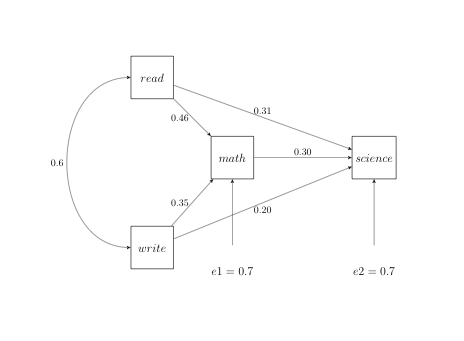
We will focus our attention on the bolded parts of the output above which include the standardized results for path list, standardized results for variance parameters and the standardized effects on science. We will use the standardized estimates as our path coefficients and the square root of the variance estimates for the error. The error values are sqrt(0.48469) = .69619681 (approx = 0.7) for math and sqrt(0.50006) = .70714921 (approx = 0.7) for science. Now we can add the path coefficients and errors to the path diagram as shown below.
The proc calis also provides estimates of the direct, indirect and total effect for the two exogenous variables because we included the effpart substatement in our model. From these results we see that the indirect effect of read is about one third that of the direct effect. While for write the indirect effect is a bit more than half the size of the direct effect. For this example, the estimates for all of the direct and indirect effects were statistically significant. This is not necessarily a very common occurrence.