First off, let’s start with what a significant three-way interaction means. It means that there is a two-way interaction that varies across levels of a third variable. Say, for example, that a b*c interaction differs across various levels of factor a.
One way of analyzing the three-way interaction is through the use of tests of simple main-effects, e.g., the effect of one variable (or set of variables) across the levels of another variable.
We will use a small artificial dataset called threeway that has a statistically significant three-way interaction to illustrate the process. In our example dataset, variables a, b, and c are categorical. The techniques shown on this page can be generalized to situations in which one or more variables are continuous, but the more continuous variables that are involved in the interaction, the more complicated things get.
In our model we have three independent variables, a, b, and c, and we believe that there is a three-way interaction. First we need to test whether there is a significant three-way interaction.
proc glm data = threeway;
  class a b c;
  model y = a|b|c;

run;
quit;

(output omitted)

      Source                      DF       Type I SS     Mean Square    F Value    Pr > F

      A                            1     150.0000000     150.0000000     112.50    <.0001
      B                            1       0.6666667       0.6666667       0.50    0.4930
      A*B                          1     160.1666667     160.1666667     120.12    <.0001
      C                            2     127.5833333      63.7916667      47.84    <.0001
      A*C                          2      18.2500000       9.1250000       6.84    0.0104
      B*C                          2      22.5833333      11.2916667       8.47    0.0051
      A*B*C                        2      18.5833333       9.2916667       6.97    0.0098

(output omitted)
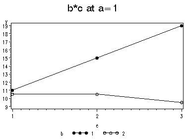
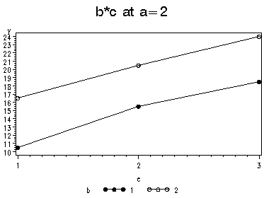
The A*B*C* interaction is statistically significant. Next, we need to select a two-way interaction to look at more closely. For the purposes of this example we will examine the b*c interaction. Let's graph the b*c interaction for each of the two levels of a. We will do this by computing the cell means for the 12 cells in the design.
proc means data=threeway;
class a b c ;
output out=means mean=ym;
var y;
types a*b*c;
run;

symbol1 color=black
        interpol=join
        value=dot
        height=1;
symbol2 color=black
        interpol=join
        value=circle
        height=1;

title1 'b*c at a=1';
proc gplot data=means;
	plot ym*c=b ;
	where a =1;
run;
quit;

title1 'b*c at a=2';
proc gplot data=means;
	plot ym*c=b;
	where a=2;
run;
quit;

We believe from looking at the two graphs above that the three-way interaction is significant because there appears to be a "strong" two-way interaction at a = 1 and no interaction at a = 2. Now, we just have to show it statistically using contrasts. The contrast statements test that the difference between levels of c is the same across levels of b. The values following the contrast statements form vectors by which the matrix of means is multiplied. It does this by comparing the pairwise difference between the means of the categories of the third variable (c), across the values of the second variable (b). The null hypothesis is that the difference across the levels of the second variable (the difference of differences) is equal to zero. In the code below, the first row of the first contrast statement tests for the difference between the means for c=1 versus c=3, and compares this difference when b=1 and b=2 (holding a=1). The second line of the first contrast statement does the same for c=2 versus c=3. The second contrast statement does the same holding a=2. After the word contrast, the information between the single quotation marks is the title, used as a label, what appears next is the effect to which the contrast is to be applied (e.g. "a" or in this case "b*c"). Following that, there is one value for each level of the variable, or in this case variables, in the effect. In the case of b*c, b has two levels, and c has three, so there are six possible combinations for the values of a*b, and hence, six values follow. Next on the line of the contrast statement is the next effect we want to include in our test, the a*b*c interaction. The first six values in the list are the same as those values for the first effect, because they are part of the interaction we are testing. The first six values apply to means for a=1, the second six, for a=2. Hence, in the first contrast statement, these values are always equal to zero. (For more information on contrasts see our page SAS FAQ: How can I do ANOVA contrasts?)
proc glm data = threeway;
class a b c;
model y = a|b|c;
contrast 'b*c at a=1' b*c 1 0 -1 -1 0 1 a*b*c 1 0 -1 -1 0 1 0 0 0 0 0 0,
                      b*c 0 1 -1 0 -1 1 a*b*c 0 1 -1 0 -1 1 0 0 0 0 0 0;
contrast 'b*c at a=2' b*c 1 0 -1 -1 0 1 a*b*c 0 0 0 0 0 0 1 0 -1 -1 0 1,
                      b*c 0 1 -1 0 -1 1 a*b*c 0 0 0 0 0 0 0 1 -1 0 -1 1;
run;
quit;


(output omitted)

Dependent Variable: Y   y

      Contrast                    DF     Contrast SS     Mean Square    F Value    Pr > F

      b*c at a=1                   2     40.66666667     20.33333333      15.25    0.0005
      b*c at a=2                   2      0.50000000      0.25000000       0.19    0.8314
Although we have rerun proc glm to perform the contrasts, we have omitted that portion of the output because it is the same as the output above. The F-ratio for the b*c interaction, when a=1 is 15.25, and the F-ratio for the b*c interaction when a=2 is 0.19. Based on the p-values presented in the output, the b*c interaction is statistically significant when a=1, but not when a=2.
In an ideal world we would be done now, but since we live in the "real" world, there is still more to do because we now need to try to understand the significant two-way interaction at a = 1; first for b = 1 and then for b = 2. This time we will use the lsmeans command, to test the a*b*c interaction, the slide=a*b option is important, since it tells SAS to compare the values of c across all values in the a*b interaction.
proc glm data = threeway;
  class a b c;
  model y = a|b|c;
  lsmeans a*b*c / slice=a*b tdiff adjust=T;
run;
quit;

(output omitted)
                                       The GLM Procedure
                                      Least Squares Means

                                                             LSMEAN
                            A    B    C        Y LSMEAN      Number

                            1    1    1      11.0000000           1
                            1    1    2      15.0000000           2
                            1    1    3      19.0000000           3
                            1    2    1      10.5000000           4
                            1    2    2      10.5000000           5
                            1    2    3       9.5000000           6
                            2    1    1      10.5000000           7
                            2    1    2      15.5000000           8
                            2    1    3      18.5000000           9
                            2    2    1      16.5000000          10
                            2    2    2      20.5000000          11
                            2    2    3      24.0000000          12


                              Least Squares Means for Effect A*B*C
                            t for H0: LSMean(i)=LSMean(j) / Pr > |t|

                                     Dependent Variable: Y

    i/j              1             2             3             4             5             6

       1                     -3.4641       -6.9282      0.433013      0.433013      1.299038
                              0.0047        <.0001        0.6727        0.6727        0.2183
       2      3.464102                     -3.4641      3.897114      3.897114       4.76314
                0.0047                      0.0047        0.0021        0.0021        0.0005
       3      6.928203      3.464102                    7.361216      7.361216      8.227241
                <.0001        0.0047                      <.0001        <.0001        <.0001
       4      -0.43301      -3.89711      -7.36122                           0      0.866025
                0.6727        0.0021        <.0001                      1.0000        0.4035
       5      -0.43301      -3.89711      -7.36122             0                    0.866025
                0.6727        0.0021        <.0001        1.0000                      0.4035
       6      -1.29904      -4.76314      -8.22724      -0.86603      -0.86603
                0.2183        0.0005        <.0001        0.4035        0.4035


(output omitted)
                                      Least Squares Means

                               A*B*C Effect Sliced by A*B for Y

                                       Sum of
             A    B        DF         Squares     Mean Square    F Value    Pr > F

             1    1         2       64.000000       32.000000      24.00    <.0001
             1    2         2        1.333333        0.666667       0.50    0.6186
             2    1         2       65.333333       32.666667      24.50    <.0001
             2    2         2       56.333333       28.166667      21.12    0.0001


NOTE: To ensure overall protection level, only probabilities associated with pre-planned
      comparisons should be used.
Again, the original ANOVA tables, along with most of the output from lsmeans has been omitted. The first table in the above output shows the means of y at different combinations of a, b, and c. The information we are really interested in appears at the very end of the output, in the table immediately above this paragraph, titled "A*B*C* Effect Sliced by A*B for Y." This table shows significance tests for differences across the three levels of c, when a and b are at various values. The first two rows are of interest, the F value of 24.00 is statistically significant (p<0.05), indicating that the mean of y varies across levels of c, when a=1 and b=1. The test of simple main-effects of was not significant when a=1 and b=2. You may be tempted to interpret the next two rows (for a=2), however, since we already tested for a b*c interaction when a=2, and found it to be non-significant, we cannot interpret these tests. But we're not done yet, since there are three levels of c, we don't know where this significant effect lies. We need to test the pairwise comparisons among the three means.
The table titled "Least Squares Means for Effect A*B*C" displays the pairwise tests for differences in the mean of c across all combinations of a, b, and c (note this table is labeled based on the numbering in column "LSMEAN number" in the table above it). These differences are given in standardized form, that is, the difference in means divided by the square root of the MSE. For example, for c=1 versus c=2 (with a=1 and b=1) we get (11-15)/sqrt(1.33)=-3.46, which is a statistically significant difference (p < 0.0047). This table gives all pairwise comparisons, however, we only want to look at the comparisons we are interested in, which is the levels of c, when a=1 and b=1, since that is where we have observed the interaction. To make this page more readable, most of this table has been omitted, but that is not a problem because the comparisons we are interested in appear in the first two rows of the table. Without correcting for multiple tests, all three of these comparisons are statistically significant. If you wish to control for multiple tests, this can be done manually.
Hopefully, we now have a much better understanding of the three-way a*b*c interaction.
Please note that the process of investigating the three-way interactions would have be similar if we had chosen a different two-way interaction back at the beginning.
Summary of Steps
1) Run full model with three-way interaction.
2) Use contrast statement to test for a two-way interaction at each level of third variable.
3) Use lsmeans, with the slice option to test for differences in the outcome at each level of second variable.
4) Run pairwise or other post-hoc comparisons if necessary
References
Kirk, Roger E. (1995) Experimental Design: Procedures for the Behavioral Sciences, Third Edition. Monterey, California: Brooks/Cole Publishing.
