Measured responses to a set range of doses is a common form of data in medicine and pharmaceutical statistics. Fitting a function to these points allows for estimating expected responses at different doses and are used to determine what levels are considered most effective and what levels might be considered toxic.
When the measured response is binary, the logistic or probit regression can be used to generate a dose response curve. See our Data Analysis Example pages for logistic and probit regression for details on each of these.
If the measured response is continuous (cell counts, hormone concentrations, etc.), then a logistic model with three or more parameters would be appropriate. On this page, we will illustrate the four-parameter logistic model often referred to as an Emax model. There are several slightly different versions of this model. We will demonstrate the parameterization shown in Pharmaceutical Statistics Using SAS: A Practical Guide by Dmitrienko et al. for the expected response, Y, given a dose, X.

There are four thetas estimated in this model: 3 and 4 are the maximum and minimum response levels, 1 is the concentration where the response is the midpoint between the maximum and minimum (sometimes referred to as ED50), and 2 is the slope parameter, indicating the speed with which the curve rises between the minimum and maximum.
We can look at a small example dataset and fit these four parameters. We will use the nlin procedure in SAS and will need to look at some summary statistics on our dose and response variables to provide reasonable starting values to the procedure. For the starting values of our maximum and minimum response, we can use the actual maximum and minimum values. For the ED50, the median or mean of the doses can be used as a starting value. And 1 is generally a reasonable starting value for the slope parameter.
data dr; input concentration response;
datalines;
.1	21.125
.1	20.575
.25	40.525
.5	26.15
.75	26.35
.75	44.275
1	49.725
1	63.6
10	49.35
10	68.875
100	58.025
100	58.075
1000	68.025
1000	52.3
;


proc means data = dr max min median;
run;

The MEANS Procedure

Variable              Maximum         Minimum          Median
-------------------------------------------------------------
concentration         1000.00       0.1000000       1.0000000
response           68.8750000      20.5750000      49.5375000
-------------------------------------------------------------

proc nlin data = dr;
  parms top = 68.875 bottom = 20.575 EC50 = 1 hill = 1;
  model response = top + (bottom - top) /
  (1 + (concentration / EC50)**hill);
run;

                                  Sum of        Mean               Approx
Source                    DF     Squares      Square    F Value    Pr > F

Model                      3      2915.8       971.9      11.64    0.0013
Error                     10       835.2     83.5176
Corrected Total           13      3751.0

The NLIN Procedure

                              Approx
Parameter      Estimate    Std Error    Approximate 95% Confidence Limits

top             59.1022       3.7306     50.7900     67.4144
bottom          27.0807       4.5930     16.8468     37.3146
EC50             0.8171       0.0884      0.6201      1.0141
hill            12.4058      11.8429    -13.9818     38.7933
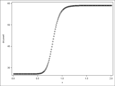
Using these four parameter estimates, we can find predicted responses for more dose levels than the original 8 and plot the dose response curve.
data a;
  x=.01;
  do i=0 to 200;
    drcurve4 = 59.1022 + ( 27.0807 - 59.1022)/(1 + (x/0.8171)**12.4058);
	output;
	x=x+.01;
  end;
run;

proc sgplot data = a;
  scatter x = x y = drcurve4;
run;

If any of the estimated values are not variable (like a minimum of zero, a maximum of 100, or a slope of one), the proc nlin code can be modified to fit a three parameter model. Most typically, the slope is constrained to one and the minimum, maximum, and ED50 are estimated.
The four parameter Emax model assumes a symmetry to the curve. The estimated value of ED50 is the inflection point of the curve at which this symmetry occurs. However, if you wish to NOT assume a symmetric curve, a five parameter logistic model is an option. In such a model, the denominator of the fraction in the four parameter model is raised to a fifth parameter. Adding a fifth parameter to our proc nlin would result in the code below:
proc nlin data = dr;
  parms top = 68.875 bottom = 20.575 EC50 = 1 hill = 1 theta5 = 1;
  model response = top + (bottom - top) /
  ((1 + (concentration / EC50)**hill)**theta5);
run;
However, this model is far more difficult to fit than the four parameter model. With our small dataset, SAS is unable to quickly converge on stable estimates. For a thorough comparison on the difference between four and five parameter models, see "The five-parameter logistic: A characterization and comparison with the four parameter logistic", 2005, by Gottschalk and Dunn.
References
Dmitienko, A., Chuang-Stein, C., D’Agostino, B. 2007. Pharmaceutical statistics using SAS: a practical guide.
Cary: SAS Publishing.
Gottschalk, P. and Dunn, J. 2005. “The five-parameter logistic: A characterization and comparison with the four-parameter logistic”, Analytical Biochemistry,
343, 1, p54-65.
