How can I generate a map in SAS using an external shape file?

Given a dataset in which variables are measured within a given area (state, country, zip code, county), the data can be presented in a map. Proc gmap in SAS provides a mechanism for going from a table of data to a map. SAS is equipped with a large number of map datasets in which the names/identifying codes and outlines of areas are defined. One can access these maps datasets by clicking on the "Maps" folder in the Explorer. Code for creating a map using one of these datasets can be found in the SAS Code Fragment: Making maps with proc gmap.

In this page, we will present how to create a map in SAS with areas defined from an imported shape file. We have a dataset, incidents, in which incidents are measured within a Los Angeles area zip code. There are multiple observations for some zip codes and other zip codes do not appear in our dataset. We wish to calculate the total number of incidents within each zip code and create a map that is color-coded according to this sum.

The Shape Data

We will need to provide SAS with data defining the zip code areas. Such a dataset can be downloaded from the Census Bureau’s website. First, download zt06_d00_shp.zip and then extract the files. The .shp file will be the one we provide to SAS. Reading it in using proc mapimport, we can indicate to SAS the nature of the file and create a dataset that can be used with proc gmap.


/* Defining our .shp file as a map in SAS */
proc mapimport datafile="C:zt06_d00.shp" out=mymap;
  select name;
run;

proc print data = mymap (obs = 10); run;


Obs        X          Y       SEGMENT    NAME

  1    -122.682    41.9148       1       96044
  2    -122.678    41.9153       1       96044
  3    -122.675    41.9170       1       96044
  4    -122.676    41.9292       1       96044
  5    -122.675    41.9308       1       96044
  6    -122.678    41.9338       1       96044
  7    -122.681    41.9367       1       96044
  8    -122.684    41.9343       1       96044
  9    -122.691    41.9342       1       96044
 10    -122.693    41.9346       1       96044

In this dataset, each observation corresponds to a discontinuity in the outline of the area. The X and Y variables indicate where the discontinuity is, SEGMENT indicates how many shapes are outlined as part of the same area, and NAME indicates the zip code.

Opening the file maps.us from the provided datasets in SAS allows for an intuitive look at this type of data. Rectangular (or nearly rectangular) states like Wyoming and North Dakota can be described with just a few observations while states with irregular borders require more points to define their perimeter. When a state is composed of multiple areas, like Michigan and Hawaii, the segment value indicates which observations correspond to which area.

Combining datasets

Once the shape file has been successfully read in and defined as a map, we can combine our data observed at the zip code level with the map. We will want to be able to match the zip code variable in both datasets together, so we first look at the contents of our map dataset to note the format and match it in our dataset. Then we use proc sql to create a new dataset with one observation for each zip code that appears in our dataset with the sum of the incident variable. Zip codes in the vicinity that do not appear in our dataset may appear as gaps in our map since we are not observing anything about them.

proc contents data = mymap; 
run;

#    Variable    Type    Len
4    NAME        Char     90
3    SEGMENT     Num       8
1    X           Num       8
2    Y           Num       8

data mydata; set "C:incidents";
  name = input(zipcode, $90.);
run;

proc sql;  
  create table zip_y as
  select distinct sum(incident) as y, name
  from mydata
  group by name;
quit;

Creating the map

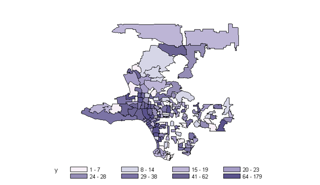
In proc gmap, we provide both a dataset and a map. The variable name identifies the area IDs. The choro statement indicates that the areas should be color-coded according to the value of y.

proc gmap data = zip_y map=mymap;
  id name;
  choro y;
run;
quit;

We may wish to change the number of levels shown and indicate values for each level. We can do this with the midpoints and range options.


proc gmap data = zip_y map=mymap;
  id name;
  choro y / midpoints = 10 35 120 range;
run;
quit;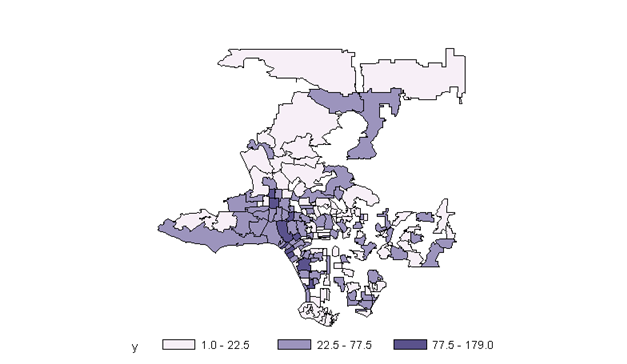

There are many other options for map features. See the SAS gallery of maps for many examples with links to code.

How can I generate a map in SAS using an external shape file? | SAS FAQ

The Shape Data

Combining datasets

Creating the map

References and resources