After running a logistic model with multiple predictors or an interaction, you may wish to be able to see predicted values with confidence intervals for different combinations of predictors. This can easily be done with the adjust command in Stata (see Stata FAQ: How do I use adjust in probit or logit?). This page will demonstrate how to achieve this in SAS by combining the outmodel and inmodel options in proc logistic with a few data steps. We will be using the hsb2.sas7bdat dataset.
data hsb2; set indata.hsb2;
  honcomp = (write >=60);
run;
Example 1: Main effect with a continuous covariate
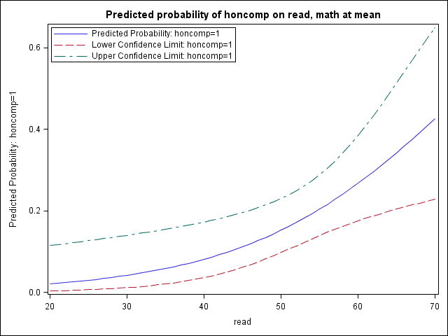
First let’s consider a logistic regression with two continuous covariates. In the regression output below, we see that both read and math are significant. We have also included outmodel in our regression so that we can save the regression parameters and apply them to another dataset. Let us focus on visualizing the effect of read when math is held at its mean.
proc logistic data = hsb2 outmodel=pout;
	model honcomp = read math;
run;

...< some output omitted >...

The LOGISTIC Procedure

             Analysis of Maximum Likelihood Estimates
                               Standard          Wald
Parameter    DF    Estimate       Error    Chi-Square    Pr > ChiSq
Intercept     1     11.9251      1.7168       48.2483        <.0001
read          1     -0.0709      0.0259        7.4891        0.0062
math          1     -0.1266      0.0305       17.1745        <.0001
We can use proc sql to generate a macro variable that is equal to the mean of math and then use a do-loop over a range of possible read values to create a dataset toscore that contains combinations of predictor variable values for which we are interested in predicted probabilities.
proc sql;
  select mean(math) into :mmath
  from hsb2;
quit;

data toscore;
  do read = 20 to 70;
   math = &mmath;
   output;
  end;
run;

proc print data = toscore (obs = 10);
run;

Obs    read     math
  1     20     52.645
  2     21     52.645
  3     22     52.645
  4     23     52.645
  5     24     52.645
  6     25     52.645
  7     26     52.645
  8     27     52.645
  9     28     52.645
 10     29     52.645
We can again run proc logistic, this time referring back to the regression parameters we saved in the first run with the inmodel option. We indicate the dataset to which the model should be applied (toscore) and the values (predicted probability with score, confidence intervals with clm) we wish to include in the generated dataset (pred). Lastly, we graph the predicted probabilities and the confidence intervals that we generate.
proc logistic inmodel=pout;
  score clm data = toscore out=pred ;
run;

proc print data = pred (obs = 10);
run;

Obs read  math  I_honcomp   P_0      P_1    LCL_0   UCL_0    LCL_1   UCL_1
  1  20  52.645     0     0.97905 0.020954 0.88499 0.99649 0.003512 0.11501
  2  21  52.645     0     0.97754 0.022459 0.88275 0.99604 0.003958 0.11725
  3  22  52.645     0     0.97593 0.024069 0.88047 0.99554 0.004460 0.11953
  4  23  52.645     0     0.97421 0.025792 0.87813 0.99497 0.005025 0.12187
  5  24  52.645     0     0.97236 0.027635 0.87574 0.99434 0.005660 0.12426
  6  25  52.645     0     0.97039 0.029606 0.87329 0.99363 0.006374 0.12671
  7  26  52.645     0     0.96829 0.031713 0.87079 0.99282 0.007177 0.12921
  8  27  52.645     0     0.96604 0.033964 0.86823 0.99192 0.008078 0.13177
  9  28  52.645     0     0.96363 0.036369 0.86560 0.99091 0.009091 0.13440
 10  29  52.645     0     0.96106 0.038937 0.86291 0.98977 0.010226 0.13709

proc sgplot data=pred;
  title "Predicted probability of honcomp on read, math at mean";
  series x=read y=P_1;
  series x=read y=LCL_1;
  series x=read y=UCL_1;
  keylegend / across = 1 location=inside position=topleft;
run;
quit;

Example 2: Categorical-by-continuous interaction with a continuous covariate
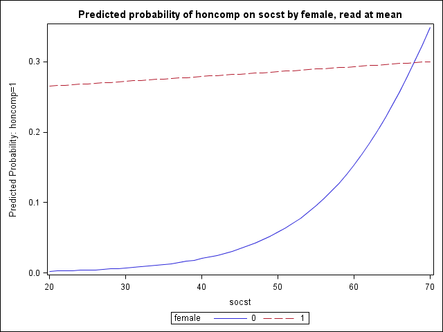
Next we consider a logistic regression where we have a significant categorical-by-continuous interaction that we wish to better understand. Our outcome is again honcomp and our model suggests that the relationship between socst and honcomp differs by level of female. We can hold our other covariate read at its mean and look at the predicted probability of honcomp on socst by female.
The overall process is the same as in Example 1. We are simply adding another do-loop when we generate toscore2, our dataset of predictor value combinations, so that we cycle through values of socst for both female = 0 and female = 1. In the plot, we leave out confidence intervals for a clearer picture (though they could easily be added).
proc logistic data = hsb2 outmodel=pout2;
	model honcomp = female|socst read;
run;
...< some output omitted >...

The LOGISTIC Procedure

               Analysis of Maximum Likelihood Estimates
                                  Standard          Wald
Parameter       DF    Estimate       Error    Chi-Square    Pr > ChiSq
Intercept        1     14.7664      2.9554       24.9648        <.0001
female           1     -7.1249      3.1138        5.2357        0.0221
socst            1     -0.1084      0.0470        5.3286        0.0210
female*socst     1      0.1050      0.0526        3.9861        0.0459
read             1     -0.1255      0.0277       20.4930        <.0001


proc sql;
  select mean(read) into :mread
  from hsb2;
quit;

data toscore2;
  do female = 0 to 1;
    do socst = 20 to 70;
     read = &mread;
     output;
    end;
  end;
run;

proc logistic inmodel=pout2;
  score clm data = toscore2 out=pred2 ;
run;

proc sgplot data=pred2;
  title "Predicted probability of honcomp on socst by female, read at mean";
  series x=socst y=P_1 / group = female;
run;
quit;
Example 3: Continuous by continuous interaction with a continuous covariate
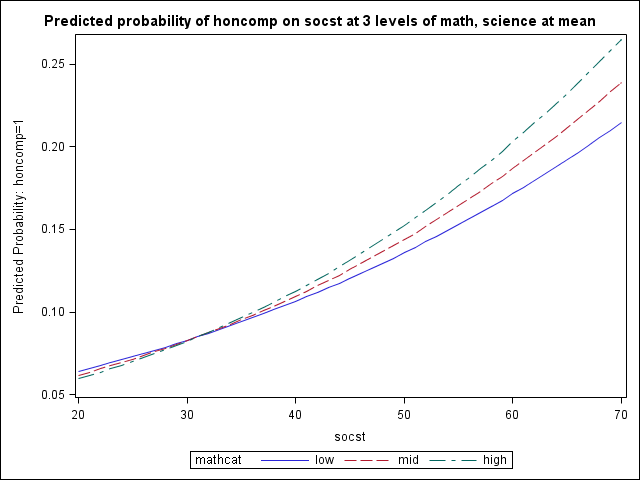
Lastly we consider a logistic regression where we have a significant continuous-by-continuous interaction and an additional covariate. Our outcome is again honcomp and our continuous variables math and socst interact significantly. We choose one of these variables (socst) to be represented continuously and we can look at its effect on the predicted probabilities of honcomp for high, mid, and low values of the other interaction variable (math). The remaining covariate (science) is held at its mean.
The overall process is the same as in Examples 1 and 2. In our toscore3 dataset, we enter our three levels of math and create an additional variable mathcat that is primarily for graphing purposes.
proc logistic data = hsb2 outmodel=pout3;
	model honcomp = math|socst science;
run;

...< some output omitted >...

The LOGISTIC Procedure

              Analysis of Maximum Likelihood Estimates
                                Standard          Wald
Parameter     DF    Estimate       Error    Chi-Square    Pr > ChiSq
Intercept      1     -3.1784      7.6480        0.1727        0.6777
math           1      0.1675      0.1449        1.3365        0.2476
socst          1      0.2523      0.1451        3.0221        0.0821
math*socst     1    -0.00539     0.00266        4.0948        0.0430
science        1     -0.0443      0.0287        2.3780        0.1231


proc sql;
  select stderr(math) into :sdmath
  from hsb2;
  select mean(science) into :mscience
  from hsb2;
quit;

data toscore3;
  do socst = 20 to 70;
    science = &mscience;
    * low math;
    math = &mmath - &sdmath;
	mathcat = "low ";
    output;
    * mean math;
    math = &mmath;
	mathcat = "mid ";
    output;
    * high math;
    math = &mmath + &sdmath;
	mathcat = "high";
    output;
  end;
run;

proc logistic inmodel=pout3;
  score clm data = toscore3 out=pred3;
run;

proc sgplot data=pred3;
  title "Predicted probability of honcomp on socst at 3 levels of math, science at mean";
  series x=socst y=P_1 / group = mathcat;
run;
quit;


