This page shows several possible uses of the predict statement in proc nlmixed. For more information about fitting models using proc nlmixed see our FAQ pages listed at the bottom of the page. Below we show how to generate predicted values for each case holding some values constant (e.g., some variables held at their mean), and finally how predict can be used with a random intercept model to get predictions that do or do not contain the random effect.
Predicted values for each case
You can download the data used in this example by clicking here: hsb2.sas7bdat.
In this example we use scores on standardized tests in writing (write), and science (science), as well as student’s gender (female) to predict scores on a standardized test of reading (read). This is a normal multiple regression (also known as OLS regression). It is not necessary to use proc nlmixed to fit this model, but it works well to demonstrate the predict statement. The SAS code to run this model using proc nlmixed appears below. After the proc nlmixed statement, we define the parameters in the model. Here xb is the linear combination of the variables used to predict read, and b0, b1, b2 and b3 are coefficients. SAS will recognize variable names and mathematical operators in these statements. Any letter, series of letters, or letter(s) followed by number(s) that are not variable names are assumed to be parameter names. Although this model only requires one line to define all the parameters, more complex models may involve more than one statement. Next we use the predict statement to record the predicted value for each case. The statement starts with predict, then gives the expression to record, in this case the predicted value of read, that is xb from the previous line. The out=output1 gives the name of the dataset (output1) in which we wish to place the predicted values. Next is the model statement. Here we define read as distributed (~) normally with mean equal to xb, and variance s2, both of which we wish to estimate (xb is estimated through the coefficients; s2 is estimated based on the model residuals).
proc nlmixed data="d:datahsb2";
   xb = b0 + b1*female + b2*write + b3*science;
   predict xb out=output1;
   model read ~ normal(xb,s2);
run;
We have omitted the output from nlmixed, since our primary interest in this FAQ is the new dataset output1. After we run the above model we can run proc contents on the dataset output1. We use the varnum option to list the variables by their order in the dataset, rather than in alphabetical order. The first eight variables (i.e., ID to SOCST) are from the dataset hsb2 that we used to estimate the above model; the rest of the variables were created by the predict statement.
proc contents data=output1 varnum;
run;

<output omitted>

                 Variables in Creation Order

 #    Variable      Type    Len    Label

 1    ID            Num       4
 2    FEMALE        Num       3
 3    RACE          Num       3
 4    SES           Num       3
 5    SCHTYP        Num       3    type of school
 6    PROG          Num       3    type of program
 7    READ          Num       3    reading score
 8    WRITE         Num       3    writing score
 9    MATH          Num       3    math score
10    SCIENCE       Num       3    science score
11    SOCST         Num       3    social studies score
12    Pred          Num       8    Predicted Value
13    StdErrPred    Num       8    Standard Error of Prediction
14    DF            Num       8    Degrees of Freedom
15    tValue        Num       8    t Value
16    Probt         Num       8    Pr > |t|
17    Alpha         Num       8    Alpha
18    Lower         Num       8    Lower Confidence Limit
19    Upper         Num       8    Upper Confidence Limit
Let’s take a closer look at the new variables. The code below uses proc print to print the values of the 8 new variables for the first 10 observations. The variable Pred contains the predicted value for each case, StdErrPred contains the standard error of that prediction. The variables tValue, and Probt contain the t-value and p-value for a test that the predicted value (Pred) is equal to zero, the degrees of freedom for this test are shown in the variable DF. The variables Lower and Upper contain the upper and lower bounds of the confidence interval for the predicted value. Alpha contains the alpha level for the confidence interval, and alpha of 0.05 corresponds to a 95% confidence interval.
proc print data=output1 (obs=10);
   var pred stderrpred df tvalue probt alpha lower upper;
run;
StdErr Obs Pred Pred DF tValue Probt Alpha Lower Upper 1 63.2338 1.13727 200 55.6013 1.3424E-123 0.05 60.9912 65.4763 2 45.1094 0.96035 200 46.9717 5.4564E-110 0.05 43.2157 47.0032 3 37.5781 1.35648 200 27.7026 2.19543E-70 0.05 34.9032 40.2529 4 51.0225 0.70175 200 72.7070 8.5867E-146 0.05 49.6387 52.4063 5 44.2521 0.93671 200 47.2423 1.9008E-110 0.05 42.4050 46.0992 6 45.1268 0.86562 200 52.1325 2.3098E-118 0.05 43.4199 46.8337 7 41.3422 1.05910 200 39.0351 1.71071E-95 0.05 39.2537 43.4306 8 42.2548 0.97955 200 43.1368 2.9686E-103 0.05 40.3233 44.1864 9 44.8790 0.94246 200 47.6190 4.417E-111 0.05 43.0206 46.7375 10 49.0661 1.21092 200 40.5197 2.25591E-98 0.05 46.6782 51.4539
Predicted values holding the values of some variables constant
This example uses the dataset used in the previous section.
You can also request predicted values holding one or more of the variables in the model constant, and using the actual value from each case for other variables. In the example below we hold write at its mean (52.775), female at one, and use each student’s science score to calculate the predicted values. This allows us to examine how predicted values of read change as the student’s science score changes, holding writing scores and gender constant. Further below we show some ways to use this information.
The code below is the same as above except for the predict statement. This time, instead of simply specifying that we want predicted values of xb we write out the regression equation, this is necessary in order to fix the values of some of the variables. In the predict statement, the variable name female has been replaced with a 1, and the variable name write has been replaced with the value 52.774 (its mean). This fixes these values to a constant for the purpose of calculating predicted values. Only the variable name science remains in the equation, so that each case’s value on this variable will be used to calculate the predicted values. The results of this predict statement are placed in the dataset output2.
proc nlmixed data="d:datahsb2";
   xb = b0 + b1*female + b2*write + b3*science;
   predict  b0 + b1*1 + b2*52.775 + b3*science out=output2;
   model read ~ normal(xb,sd);
run;
Using the predicted values in output2 we can calculate the predicted mean of read for female students with average writing scores, and the sample values for science. The average predicted reading score, holding writing score and gender constant, while allowing science to vary is 51.23, with a standard deviation of 3.95.
proc means data=output2;
   var pred;
run;

                        The MEANS Procedure

              Analysis Variable : Pred Predicted Value

  N            Mean         Std Dev         Minimum         Maximum

200      51.2252437       3.9549304      40.8994103      60.0731049
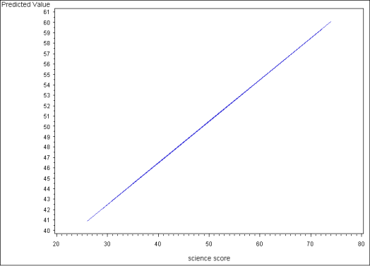
The predicted values can also be used to graph the relationship between science and predicted values of read, holding the other variables constant (if the other variables in the model aren’t held constant, the result will not be a single regression line, but a scattering of points). Below we use proc gplot to generate a line graph showing this relationship. The first line of code below clears previous graph setting, the second instructs SAS to connect the data points to form a line, rather than graphing a series of unconnected points. Next is the proc gplot statement, on which we tell SAS that we want to create a graph using the dataset output2. The plot statement instructs SAS to graph pred against science. Finally, run; executes the command and quit; instructs SAS that we will not be working with this graph further. (For more information on proc gplot, see our SAS Learning Module: Graphing data in SAS.)
goptions reset=all border;
symbol1 interpol=join;

proc gplot data=output2;
   plot pred*science;
run;
quit;
Below we show the resulting graph. This graph shows the predicted values of read across the observed values of science, holding write at its mean and female at one. Since this is a linear model, with no interaction terms, if we used other values of write and/or female, the predicted values would be different, but the slope of the line would be the same.

Predict in a model with a random intercept
You can download the data used in this example by clicking here: https://stats.idre.ucla.edu/wp-content/uploads/2016/02/hsb-1.sas7bdat.
In this example we show how the predict statement can be used in a model with random effects. The dataset for this example includes information on 7185 students in 160 schools. (Note: this dataset comes from the HLM manual.) The variable mathach is a measure of each student’s math achievement, the variable female is a binary variable equal to one if the student is female and zero otherwise, and the variable pracad is a school level variable, the proportion of students at each school who are on an academic track. The variable id identifies which school a student attends. In the model we use female and pracad to predict mathach, and include a random intercept for schools.
The first line of code below begins the proc nlmixed command. The second line specifies the conditional mean of mathach for student i in classroom j as a linear combination of the fixed and random effects, and calls this value mu_ij. The third line specifies that the random term be called u_j. The model statement specifies that mathach is distributed (~) normally with a mean of mu_ij and residual variance sigma2. The random statement defines the random effect u_j as normally distributed with mean zero and a variance term, tau2, to be estimated. The level 2 units, schools, are identified by subject=id;. The last two lines of the command are predict statements. The first predict statement gives us the predicted means for each observation based on the fixed and random effects, identified by mu_ij, and outputs a dataset called output_fixed_and_random. The second predict statement generates predicted values that include the estimate of the random intercept in addition to the fixed portion of the model. To get the predictions using only the fixed effects, subtract the predictions in output_random from the predictions in output_fixed_and_random.
proc nlmixed data="d:datahsb";
   mu_ij = b0 + u_j + female*b1 + pracad*b2;
   rand = u_j;
   model mathach ~ normal(mu_ij,sigma2);
   random u_j ~ normal(0,tau2) subject=id;
   predict  mu_ij out=output_fixed_and_random;
   predict  rand out=output_random;
run;
Using predicted values to calculate and graph residuals
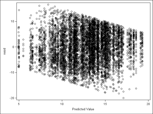
We can use the predicted value is to calculate residuals. Using the dataset output_random from the previous example, the data step below calculates the residuals by subtracting each student’s predicted mathach score (xb) from their actual score (mathach), creating a new variable resid. This example calculates residuals for the dataset where the predicted values include the random intercept (output_random), however, depending on our purpose, we also could have used the dataset with only the fixed effects (output_fixed). After calculating the residuals we use proc sgplot to plot the residuals (resid) versus fitted values (pred) in a scatterplot.
data output_random;
	set output_random ;
	resid=mathach-pred;
run;

proc sgplot data=output_random;
	scatter x=pred y=resid;
run;

See Also
- SAS FAQ: How can I run simple linear and nonlinear models using nlmixed?
- SAS FAQ: From an OLS model to full mixed models using proc nlmixed
