NOTE: As of SAS 9.2, the histogram statement in
proc univariate will now by default direct graphs to
ODS graphics rather than “tradtional graphics”. Many old options, such
as cfill=, which was used to change the color of the
histogram bars, are ignored by ODS graphics and have been replaced
by style options that can be set in proc template.
Previous versions of this page used traditional graphics, the code
for which we have preserved at the bottom of the page. The page
has been updated for SAS 9.3 with creation of histograms with
percentages on the bars using ODS graphics.
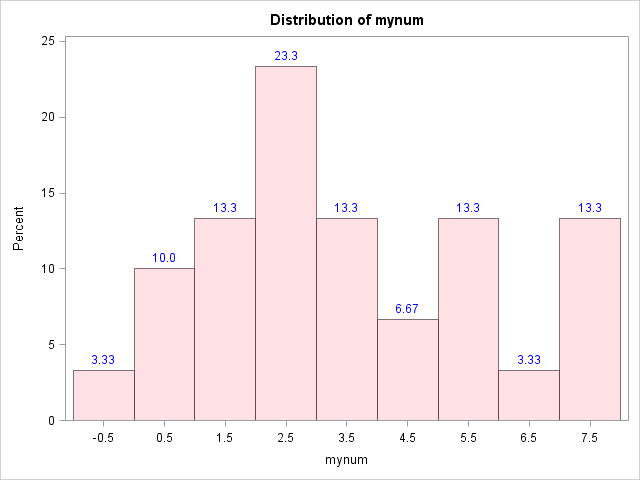
Consider this simple data file with a variable called mynum. We are going to create a histogram of mynum with percentages on top of each bar.
data test;
  input mynum @@;
  cards;
  2.3 -.6
  3.3 3.5
  2.4 5.6
  7.8 2.4
  2.8 4.5
  6.3 1.2
  0.5  .8
  .9  1.2
  1.4 1.5
  2.3 2.5
  2.7 3.5
  3.1 4.6
  5.5 5.8
  5.3 7.6
  7.3 7.8
;
run;
Let’s say the midpoints that we are going to
use for our histogram are -.5, 1.5, … 7.5, since the range of the variable
is between -1 to 8. The width of each bin is 1. Below in a data step, a variable called
ind is
created as a group variable representing each bin (bar). Then we use proc
freq with ods output option to output the frequencies and
percentages to a dataset called temp3.
data temp2;
set test;
do i = -.5 to 7.5 by 1;
if i-.5 <= mynum < i+.5 then ind=i;
end;
run;
proc freq data=temp2;
tables ind ;
ods output OneWayFreqs=temp3;
run;Let’s print out the ods output data
set temp3 from proc freq.
proc print data=temp3;
run;
Cum Cum
Obs Table F_ind ind Frequency Percent Frequency Percent
1 ind -0.5 -0.5 1 3.33 1 3.33
2 ind 0.5 0.5 3 10.00 4 13.33
3 ind 1.5 1.5 4 13.33 8 26.67
4 ind 2.5 2.5 7 23.33 15 50.00
5 ind 3.5 3.5 4 13.33 19 63.33
6 ind 4.5 4.5 2 6.67 21 70.00
7 ind 5.5 5.5 4 13.33 25 83.33
8 ind 6.5 6.5 1 3.33 26 86.67
9 ind 7.5 7.5 4 13.33 30 100.00We are now ready to create our histogram with percentages on top of
each bar. We request these precentages with the option barlabel=percent in
the histogram statement. In proc
template, we define a new style newstyle that
inherits all of the specification of the SAS HTML default
style htmlblue, but we change the color of the bars and the color of the
text used to print the percentages. We then ask that SAS use this
new style with the ods html style= statement.
proc template ;
define style Styles.newstyle;
parent = Styles.htmlblue;
style GraphDataDefault /
Color = pink;
style GraphDataText /
Color = blue;
end;
run;
ods html style=Styles.newstyle;
proc univariate data=temp2 ;
histogram mynum /barlabel=percent midpoints=-.5 to 7.5 by 1;
run;

NOTE: The following text and code, created before
SAS 9.2, are from an older version of this
page, which will create the same histogram
produced above, but here in SAS “traditional graphics”. To create
this histogram with traditional graphics, so that all the options
listed here will work, the command ods graphics
off; must be issued.
Consider this simple data file with a variable called mynum. We are going to create a histogram of mynum with percentages on top of each bar.
data test;
input mynum @@;
cards;
2.3 -.6
3.3 3.5
2.4 5.6
7.8 2.4
2.8 4.5
6.3 1.2
0.5 .8
.9 1.2
1.4 1.5
2.3 2.5
2.7 3.5
3.1 4.6
5.5 5.8
5.3 7.6
7.3 7.8
;
run;Let’s say the midpoints that we are going to
use for our histogram are -.5, 1.5, … 7.5, since the range of the variable
is between -1 to 8. The width of each bin is 1. Below in a data step, a variable called
ind is
created as a group variable representing each bin (bar). Then we use proc
freq with ods output option to output the frequencies and
percentages to a dataset called temp3.
data temp2;
  set test;
  do i = -.5 to 7.5 by 1;
  if  i-.5 <= mynum < i+.5 then ind=i;
  end;
run;
proc freq data=temp2;
tables ind ;
ods output OneWayFreqs=temp3;
run;
Let’s print out the ods output data
set temp3 from proc freq.
proc print data=temp3;
run;

                                                                     Cum         Cum
         Obs    Table    F_ind     ind    Frequency    Percent    Frequency    Percent

          1      ind     -0.5     -0.5           1       3.33            1       3.33
          2      ind      0.5      0.5           3      10.00            4      13.33
          3      ind      1.5      1.5           4      13.33            8      26.67
          4      ind      2.5      2.5           7      23.33           15      50.00
          5      ind      3.5      3.5           4      13.33           19      63.33
          6      ind      4.5      4.5           2       6.67           21      70.00
          7      ind      5.5      5.5           4      13.33           25      83.33
          8      ind      6.5      6.5           1       3.33           26      86.67
          9      ind      7.5      7.5           4      13.33           30     100.00
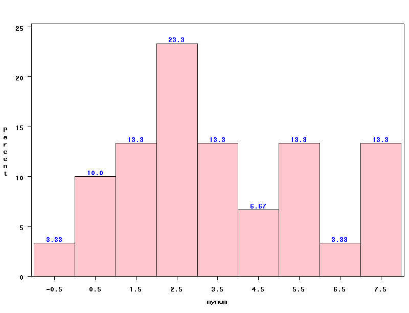
We can now use this data set to create an
annotate data set and use it with proc univariate to create the
histogram with percentage on top of each bar.
data anno;
set temp3;
length function color text $8;
function = 'label';
color = 'blue';
size = 1;
xsys = '2';
ysys = '2';
when = 'a';
x=ind; /*the x-coordinate for the text*/
y=percent+.5; /*the y-coordinate*/
text=left(put(percent, 4.2));
run;
ods graphics
  off;
proc univariate data=temp2 noprint;
histogram mynum /anno=anno cfill=pink midpoints=-.5 to 7.5 by 1;
run;
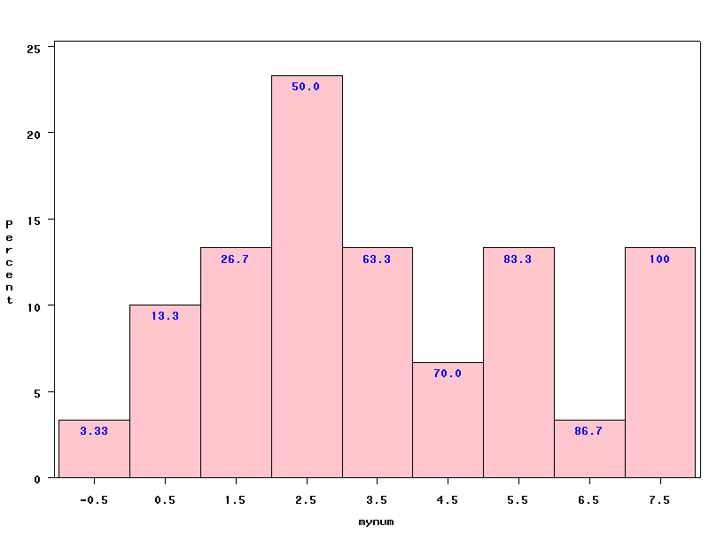
Using the same idea, we can also get a histogram with cumulative percentage on top of each bar. This time we lower the Y-axis position so the percentage is inside of the bar.
data anno;
    set temp3;
    length function color text $8;

      function = 'label';
      color    = 'blue';
      size     =  1;
      xsys     = '2';
      ysys     = '2';
      when     = 'a';
      x=ind;
      y=percent-.5;
	  text=left(put(cumpercent, 4.2));
run;

ods graphics off;

proc univariate data=temp2 noprint;
histogram mynum /anno=anno cfill=pink midpoints=-.5 to 7.5 by 1;
run;
