The ttest procedure performs t-tests for one sample, two samples and paired observations. The single-sample t-test compares the mean of the sample to a given number (which you supply). The dependent-sample t-test compares the difference in the means from the two variables to a given number (usually 0), while taking into account the fact that the scores are not independent. The independent samples t-test compares the difference in the means from the two groups to a given value (usually 0). In other words, it tests whether the difference in the means is 0. In our examples, we will use the hsb2 data set.
Single sample t-test
For this example, we will compare the mean of the variable write with a pre-selected value of 50. In practice, the value against which the mean is compared should be based on theoretical considerations and/or previous research.
proc ttest data="D:\hsb2" H0=50;
var write;
run;
The TTEST Procedure
                                         Statistics
                   Lower CL            Upper CL   Lower CL             Upper CL
Variable       N       Mean     Mean       Mean    Std Dev   Std Dev    Std Dev   Std Err
write        200     51.453   52.775     54.097     8.6318    9.4786     10.511    0.6702

                T-Tests
Variable      DF    t Value    Pr > |t|
write        199       4.14      <.0001
Summary statistics
                                         Statistics

                   Lower CL            Upper CL   Lower CL             Upper CL
Variablea      Nb      Meanc    Meand      Meanc   Std Deve  Std Devf   Std Deve  Std Errg
write        200     51.453   52.775     54.097     8.6318    9.4786     10.511    0.6702
a. Variable – This is the list of variables. Each variable that was listed on the var statement will have its own line in this part of the output.
b. N – This is the number of valid (i.e., non-missing) observations used in calculating the t-test.
c. Lower CL Mean and Upper CL Mean – These are the lower and upper bounds of the confidence interval for the mean. A confidence interval for the mean specifies a range of values within which the unknown population parameter, in this case the mean, may lie. It is given by
![]()
where s is the sample deviation of the observations and N is the number of valid observations. The t-value in the formula can be computed or found in any statistics book with the degree of freedom being N-1 and the p-value being 1-alpha/2, where alpha is the confidence level and by default is .95. If we drew 200 random samples, then about 190 (200*.95) times, the confidence interval would capture the parameter mean of the population.
d. Mean – This is the mean of the variable.
e. Lower CL Std Dev and Upper CL Std Dev – Those are the lower and upper bound of the confidence interval for the standard deviation. A confidence interval for the standard deviation specifies a range of values within which the unknown parameter, in this case, the standard deviation, may lie. The computation of the confidence interval is based on a chi-square distribution and is given by the following formula
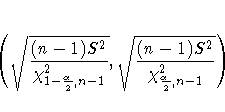
where S2 is the estimated variance of the variable and alpha is the confidence level. If we drew 200 random samples, then about 190 (200*.95) of times, the confidence interval would capture the parameter standard deviation of the population.
f. Std Dev – This is the standard deviation of the variable.
g. Std Err – This is the estimated standard deviation of the sample mean. If we drew repeated samples of size 200, we would expect the standard deviation of the sample means to be close to the standard error. The standard deviation of the distribution of sample mean is estimated as the standard deviation of the sample divided by the square root of sample size. This provides a measure of the variability of the sample mean. The Central Limit Theorem tells us that the sample means are approximately normally distributed when the sample size is 30 or greater.
Test statistics
The single sample t-test tests the null hypothesis that the population mean is equal to the given number specified using the option H0= . The default value in SAS for H0 is 0. It calculates the t-statistic and its p-value for the null hypothesis under the assumption that the sample comes from an approximately normal distribution. If the p-value associated with the t-test is small (usually set at p < 0.05), there is evidence that the mean is different from the hypothesized value. If the p-value associated with the t-test is not small (p > 0.05), then the null hypothesis is not rejected, and you conclude that the mean is not different from the hypothesized value.
In our example, the t-value for variable write is 4.14 with 199 degrees of freedom. The corresponding p-value is .0001, which is less than 0.05. We conclude that the mean of variable write is different from 50.
                T-Tests
Variablea     DFh   t Valuei   Pr > |t|j
write        199       4.14      <.0001
a. Variable – This is the list of variables. Each variable that was listed on the var statement will have its own line in this part of the output. If a var statement is not specified, proc ttest will conduct a t-test on all numerical variables in the dataset.
h. DF – The degrees of freedom for the single sample t-test is simply the number of valid observations minus 1. We loose one degree of freedom because we have estimated the mean from the sample. We have used some of the information from the data to estimate the mean; therefore, it is not available to use for the test and the degrees of freedom accounts for this.
i. t Value – This is the Student t-statistic. It is the ratio of the difference between the sample mean and the given number to the standard error of the mean. Since that the standard error of the mean measure the variability of the sample mean, the smaller the standard error of the mean, the more likely that our sample mean is close to the true population mean. This is illustrated by the following three figures.
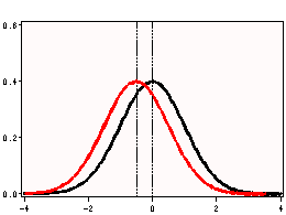
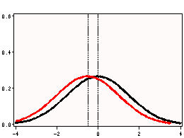
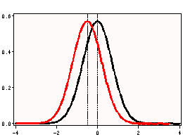
All three cases the difference between the population means are the same. But with large variability of sample means, two populations overlap a great deal. Therefore, the difference may well come by chance. On the other hand, with small variability, the difference is more clear. The smaller the standard error of the mean, the larger the magnitude of the t-value. Therefore, the smaller the p-value. The t-value takes into account of this fact.
j. Pr > |t| – The p-value is the two-tailed probability computed using t distribution. It is the probability of observing a greater absolute value of t under the null hypothesis. For a one-tailed test, halve this probability. If p-value is less than the pre-specified alpha level (usually .05 or .01) we will conclude that mean is statistically significantly different from zero. For example, the p-value for write is smaller than 0.05. So we conclude that the mean for write is significantly different from 50.
Dependent group t-test
A dependent group t-test is used when the observations are not independent of one another. In the example below, the same students took both the writing and the reading test. Hence, you would expect there to be a relationship between the scores provided by each student. The dependent group t-test accounts for this. In the example below, the t-value for the difference between the variables write and read is 0.87 with 199 degrees of freedom, and the corresponding p-value is .3868. This is greater than our pre-specified alpha level, 0.05. We conclude that the difference between the variables write and read is not statistically significantly different from 0. In other words, the means for write and read are not statistically significantly different from one another.
proc ttest data="D:\hsb2";
paired write*read;
run;
The TTEST Procedure
Statistics
                        Lower CL            Upper CL   Lower CL             Upper CL
Difference          N       Mean     Mean       Mean    Std Dev   Std Dev    Std Dev   Std Err
write - read 200 -0.694 0.545 1.7841 8.0928 8.8867 9.8546 0.6284
T-Tests
Difference DF t Value Pr > |t|
write - read 199 0.87 0.3868
Summary statistics
The TTEST Procedure
Statistics
                        Lower CL            Upper CL   Lower CL             Upper CL
Differencea         Nb      Meanc    Meand      Meanc   Std Deve  Std Devf   Std Deve  Std Errg
write - read 200 -0.694 0.545 1.7841 8.0928 8.8867 9.8546 0.6284
a. Difference – This is the list of variables.
b. N – This is the number of valid (i.e., non-missing) observations used in calculating the t-test.
c. Lower CL Mean and Upper CL Mean – These are the lower and upper bounds of the confidence interval for the mean. A confidence interval for the mean specifies a range of values within which the unknown population parameter, in this case the mean, may lie. It is given by
![]()
where s is the sample deviation of the observations and N is the number of valid observations. The t-value in the formula can be computed or found in any statistics book with the degree of freedom being N-1 and the p-value being 1-alpha/2, where alpha is the confidence level and by default is .95. If we drew 200 random samples, then about 190 (200*.95) times, the confidence interval would capture the parameter mean of the population.
d. Mean – This is the mean of the variable.
e. Lower CL Std Dev and Upper CL Std Dev – Those are the lower and upper bound of the confidence interval for the standard deviation. A confidence interval for the standard deviation specifies a range of values within which the unknown parameter, in this case, the standard deviation, may lie. The computation of the confidence interval is based on a chi-square distribution and is given by the following formula

where S2 is the estimated variance of the variable and alpha is the confidence level. If we drew 200 random samples, then about 190 (200*.95) of times, the confidence interval would capture the parameter standard deviation of the population.
f. Std Dev – This is the standard deviation of the variable.
g. Std Err – This is the estimated standard deviation of the sample mean. If we drew repeated samples of size 200, we would expect the standard deviation of the sample means to be close to the standard error. The standard deviation of the distribution of sample mean is estimated as the standard deviation of the sample divided by the square root of sample size. This provides a measure of the variability of the sample mean. The Central Limit Theorem tells us that the sample means are approximately normally distributed when the sample size is 30 or greater.
Test statistics
T-Tests
Differenceh DFi t Valuej Pr > |t|k
write - read 199 0.87 0.3868
h. Difference – The t-test for dependent groups is to form a single random sample of the paired difference. Therefore, essentially it is a simple random sample test. The interpretation for t-value and p-value is the same as for the case of simple random sample.
i. DF – The degrees of freedom for the paired observations is simply the number of observations minus 1. This is because the test is conducted on the one sample of the paired differences.
j. t Value – This is the t-statistic. It is the ratio of the mean of the difference in means to the standard error of the difference (.545/.6284).
k. Pr > |t| – The p-value is the two-tailed probability computed using t distribution. It is the probability of observing a greater absolute value of t under the null hypothesis. For a one-tailed test, halve this probability. If p-value is less than our pre-specified alpha level, usually 0.05, we will conclude that the difference is significantly from zero. For example, the p-value for the difference between write and read is greater than 0.05, so we conclude that the difference in means is not statistically significantly different from 0.
Independent group t-test
This t-test is designed to compare means of same variable between two groups. In our example, we compare the mean writing score between the group of female students and the group of male students. Ideally, these subjects are randomly selected from a larger population of subjects. Depending on if we assume that the variances for both populations are the same or not, the standard error of the mean of the difference between the groups and the degree of freedom are computed differently. That yields two possible different t-statistic and two different p-values. When using the t-test for comparing independent groups, we need to test the hypothesis on equal variance and this is a part of the output that proc ttest produces. The interpretation for p-value is the same as in other type of t-tests.
proc ttest data="D:\hsb2";
class female;
var write;
run;
The TTEST Procedure
Statistics
                               Lower CL          Upper CL  Lower CL           Upper CL
Variable  female            N      Mean    Mean      Mean   Std Dev  Std Dev   Std Dev  Std Err
write                0     91    47.975  50.121    52.267    8.9947   10.305    12.066   1.0803
write                1    109    53.447  54.991    56.535    7.1786   8.1337    9.3843   0.7791
write     Diff (1-2)             -7.442   -4.87    -2.298    8.3622   9.1846    10.188   1.3042
T-Tests
Variable Method Variances DF t Value Pr > |t|
write       Pooled           Equal         198      -3.73      0.0002
write       Satterthwaite    Unequal       170      -3.66      0.0003
Equality of Variances
Variable Method Num DF Den DF F Value Pr > F
write Folded F 90 108 1.61 0.0187
Summary statistics
Statistics
                               Lower CL          Upper CL  Lower CL           Upper CL
Variablea femaleb           Nc     Meand   Meane     Meand  Std Devf Std Devg  Std Devf Std Errh
write                0     91    47.975  50.121    52.267    8.9947   10.305    12.066   1.0803
write                1    109    53.447  54.991    56.535    7.1786   8.1337    9.3843   0.7791
write     Diff (1-2)             -7.442   -4.87    -2.298    8.3622   9.1846    10.188   1.3042
a. Variable – This column lists the dependent variable(s). In our example, the dependent variable is write.
b. female – This column gives values of the class variable, in our case female. This variable is necessary for doing the independent group t-test and is specified by class statement.
c. N – This is the number of valid (i.e., non-missing) observations in each group defined by the variable listed on the class statement (often called the independent variable).
d. Lower CL Mean and Upper CL Mean – These are the lower and upper confidence limits of the mean. By default, they are 95% confidence limits.
e. Mean – This is the mean of the dependent variable for each level of the independent variable. On the last line the difference between the means is given.
f. Lower CL Std Dev and Upper LC Std Dev – These are the lower and upper 95% confidence limits for the standard deviation for the dependent variable for each level of the independent variable.
g. Std Dev – This is the standard deviation of the dependent variable for each of the levels of the independent variable. On the last line the standard deviation for the difference is given.
h. Std Err – This is the standard error of the mean.
Test statistics
T-Tests
Variablea Methodi Variancesj DFk t Valuel Pr > |t|m
write       Pooled           Equal         198      -3.73      0.0002
write       Satterthwaite    Unequal       170      -3.66      0.0003
Equality of Variances
Variablea Methodi Num DFn Den DFn F Valueo Pr > Fp
write Folded F 90 108 1.61 0.0187
a. Variable – This column lists the dependent variable(s). In our example, the dependent variable is write.
i. Method – This column specifies the method for computing the standard error of the difference of the means. The method of computing this value is based on the assumption regarding the variances of the two groups. If we assume that the two populations have the same variance, then the first method, called pooled variance estimator, is used. Otherwise, when the variances are not assumed to be equal, the Satterthwaite’s method is used.
j. Variances – The pooled estimator of variance is a weighted average of the two sample variances, with more weight given to the larger sample and is defined to be
s2 = ((n1-1)s1+(n2-1)s2)/(n1+n2-2),
where s1 and s2 are the sample variances and n1 and n2 are the sample sizes for the two groups. the This is called pooled variance. The standard error of the mean of the difference is the pooled variance adjusted by the sample sizes. It is defined to be the square root of the product of pooled variance and (1/n1+1/n2). In our example, n1=109, n2=91. The pooled variance = 108*8.13372+90*10.3052/198=84.355. It follows that the standard error of the mean of the difference = sqrt(84.355*(1/109+1/91))=1.304. This yields our t-statistic to be -4.87/1.304=-3.734.
Satterthwaite is an alternative to the pooled-variance t test and is used when the assumption that the two populations have equal variances seems unreasonable. It provides a t statistic that asymptotically (that is, as the sample sizes become large) approaches a t distribution, allowing for an approximate t test to be calculated when the population variances are not equal.
k. DF – The degrees of freedom for the paired observations is simply the number of observations minus 2. We use one degree of freedom for estimating the mean of each group, and because there are two groups, we use two degrees of freedom.
l. t Value – This t-test is designed to compare means between two groups of the same variable such as in our example, we compare the mean writing score between the group of female students and the group of male students. Depending on if we assume that the variances for both populations are the same or not, the standard error of the mean of the difference between the groups and the degrees of freedom are computed differently. That yields two possible different t-statistic and two different p-values. When using the t-test for comparing independent groups, you need to look at the variances for the two groups. As long as the two variances are close (one is not more than two or three times the other), go with the equal variances test. The interpretation for the p-value is the same as in other types of t-tests.
m. Pr > |t| – The p-value is the two-tailed probability computed using the t distribution. It is the probability of observing a t-value of equal or greater absolute value under the null hypothesis. For a one-tailed test, halve this probability. If the p-value is less than our pre-specified alpha level, usually 0.05, we will conclude that the difference is significantly different from zero. For example, the p-value for the difference between females and males is less than 0.05, so we conclude that the difference in means is statistically significantly different from 0.
n. Num DF and Den DF – The F distribution is the ratio of two estimates of variances. Therefore it has two parameters, the degrees of freedom of the numerator and the degrees of freedom of the denominator. In SAS convention, the numerator corresponds to the sample with larger variance and the denominator corresponds to the sample with smaller variance. In our example, the male students group ( female=0) has variance of 10.305^2 (the standard deviation squared) and for the female students the variance is 8.1337^2. Therefore, the degrees of freedom for the numerator is 91-1=90 and the degrees of freedom for the denominator 109-1=108.
o. F Value – SAS labels the F statistic not F, but F’, for a specific reason. The test statistic of the two-sample F test is a ratio of sample variances, F = s12/s22 where it is completely arbitrary which sample is labeled sample 1 and which is labeled sample 2. SAS’s convention is to put the larger sample variance in the numerator and the smaller one in the denominator. This is called the folded F-statistic,
F’ = max(s12,s22)/min(s12,s22)
which will always be greater than 1. Consequently, the F test rejects the null hypothesis only for large values of F’. In this case, we get 10.305^2 / 8.1337^2 = 1.605165, which SAS rounds to 1.61.
p. Pr > F – This is the two-tailed significance probability. In our example, the probability is less than 0.05. So there is evidence that the variances for the two groups, female students and male students, are different. Therefore, we may want to use the second method (Satterthwaite variance estimator) for our t-test.
