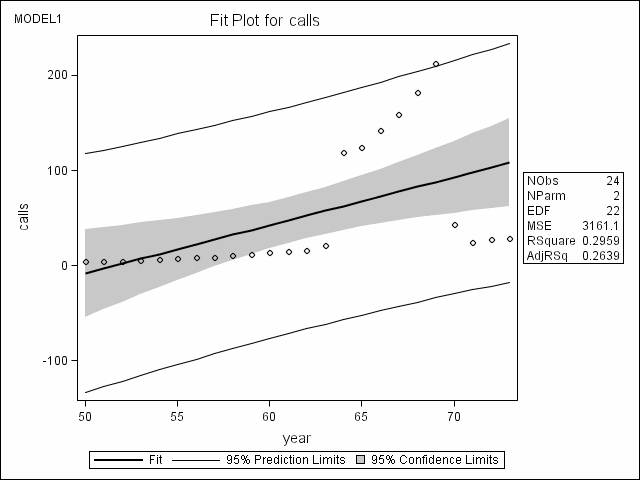
Robust regression models are often used to detect outliers and to provide stable estimates in the presence of outliers. Procedure ROBUSTREG in SAS 9 has implemented four common methods of performing robust regression. This page will show some examples on how to perform different types of robust regression analysis using proc robustreg. The examples are mainly taken from Modern Applied Statistics with S (4th edition, page 158 – 161) and the data set by Rousseeuw and Leroy on annual numbers of Belgian telephone calls, phones.sas7bdat, is used and can be downloaded here.
1. What are outliers?
Outliers are data points with extreme values in a random sample. For a regression analysis, there are basically two ways that a data point can be extreme. It can be extreme in the direction of the outcome variable (y-direction). It can also be a multivariate outlier in the predictor space (x-direction), which is also referred as a leverage point. Sometimes, an outlier can be both in the direction of the y-direction and x-direction, which is also called an influence point. Outliers can yield biased estimation of regression parameters.
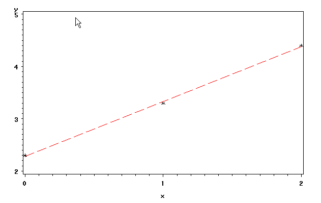
Let us take a look at some extremely simple-minded examples. Data set demo0 has three data points. We should be able to tell that by design, the regression line is close to each point and this is shown by the scatter plot below. There are no outliers in this data set.
data demo0;
  input y x;
datalines;
2.3 0
3.3 1
4.4 2
;
run;

symbol i = r v=star l=2 ci=red cv=black;
proc gplot data = demo;
  plot y*x;
run;
quit;
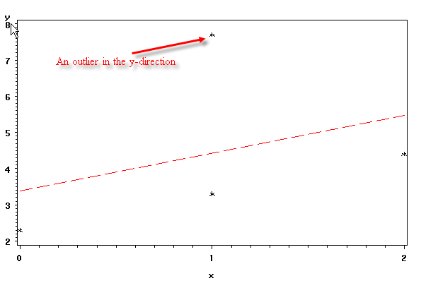
How can a point be a outlier in the direction of y? The data point simply takes extreme value in y. For example, in our next data set demo1, we have added one point (1, 7,7). In terms of x-direction, it is right in the middle, but in terms of y-direction, it is way up. You can see that the residual for this point is particular large than those of other data points. The regression line is then lifted upwards, but the slope of the regression does not change much.
data demo1;
  input y x;
datalines;
2.3 0
3.3 1
4.4 2
7.7 1
;
run;
symbol i = r v=star l=2 ci=red cv=black;
proc gplot data = demo1;
  plot y*x;
run;
quit;
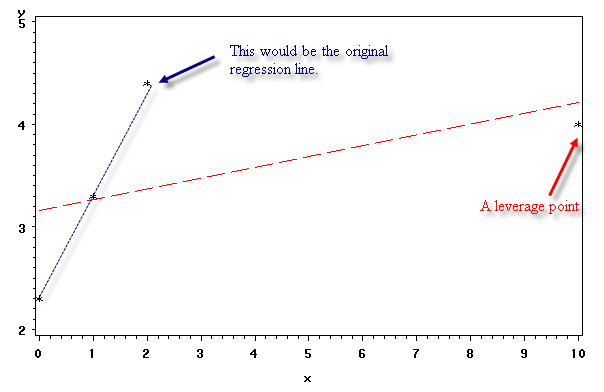
Now let us create a data point that is leverage point, that is outlier in the x-direction. We add one point (10, 4). It is extreme in the x-direction. Notice that the residual of this point is not particularly larger than that of any other points, but the slope has changed greatly. That is why outliers in the x-direction are also called leverage points, since they "leverage" the regression line.
data demo2;
  input y x;
datalines;
2.3 0
3.3 1
4.4 2
4  10
;
run;
proc gplot data = demo2;
  plot y*x;
run;
quit;
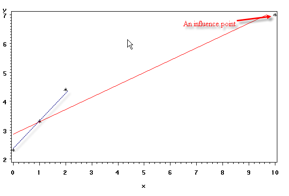
Last but not least, let us create an example with an influence point. To this end, we just need to add a point for which both the y-direction and x-direction are extreme. An influence point affects both the intercept and the slope of a regression model.
data demo2;
  input y x;
datalines;
2.3 0
3.3 1
4.4 2
7  10
;
run;

symbol1 i = r v=star cv=black ci=red;
proc gplot data = demo2;
  plot y*x;
run;
quit;
If these static examples have not satisfied your curiosity, you can play a regression applet developed by Professor West of University of South Carolina.
2. Detection of outliers and Remedies
Now we know what outliers are, the question is how to detect them and what to do after we detect them.
2. M estimation
Introduced by Huber in 1973, M-estimators have been widely used in models where outliers are in the direction of the outcome variable. Each M-estimator corresponds to a specific weight function. Some commonly used weight functions are Huber weight function and bisquare weight function. Notice that OLS regression can be considered as a special case of M-estimator, where the weight function is the identity function. The Robustreg procedure offers ten kinds of weight functions. For details on the definition of weight functions and their shapes, please visit SAS’s page on the
weight functions.
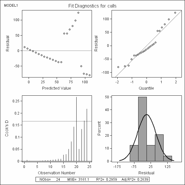
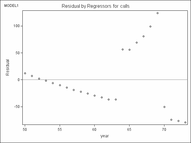
Example 1. OLS regression with identical weight function by proc reg; the first model on page 159. This example is mainly used for comparison with the robust regression models. To this end, we will also make use ODS graphics facility of SAS 9 to create diagnostics plots.
ods html style = journal;
ods graphics on;
proc reg data = phones;
  model calls = year;
run;
quit;
ods graphics off;
ods html close;
Analysis of Variance
                                    Sum of           Mean
Source                   DF        Squares         Square    F Value    Pr > F
Model                     1          29229          29229       9.25    0.0060
Error                    22          69544     3161.06999
Corrected Total          23          98773
Root MSE             56.22339    R-Square     0.2959
Dependent Mean       49.99167    Adj R-Sq     0.2639
Coeff Var           112.46553
Parameter Estimates
                                  Parameter       Standard
Variable     Label        DF       Estimate          Error    t Value    Pr > |t|
Intercept    Intercept     1     -260.05925      102.60700      -2.53      0.0189
year         year          1        5.04148        1.65794       3.04      0.0060
Example 2. M-estimator with Huber’s weight function, the second model on page 159.
proc robustreg data = phones method = m (wf=huber);
  model calls = year;
run;
The ROBUSTREG Procedure
Model Information
Data Set                              WORK.PHONES
Dependent Variable                          calls    calls
Number of Independent Variables                 1
Number of Observations                         24
Method                               M Estimation
Number of Observations Read          24
Number of Observations Used          24
Summary Statistics
                                                              Standard
Variable           Q1      Median          Q3        Mean    Deviation         MAD
year          55.5000     61.5000     67.5000     61.5000       7.0711      8.8956
calls          7.7000     15.5000     81.0000     49.9917      65.5321     15.1225
Parameter Estimates
                      Standard   95% Confidence     Chi-
Parameter DF Estimate    Error       Limits       Square Pr > ChiSq
Intercept  1 -102.530  26.4920 -154.454 -50.6067   14.98     0.0001
year       1   2.0396   0.4281   1.2006   2.8786   22.70     <.0001
Scale      1   9.0093
Diagnostics Summary
Observation
Type           Proportion      Cutoff
Outlier 0.2500 3.0000
Goodness-of-Fit
Statistic Value
R-Square       0.1780
AICR         229.6477
BICR         230.6074
Deviance     18201.95
Example 3: M-estimator with Huber’s weight and Huber’s scale, the third model on page 159.
proc robustreg data = phones method = m (scale=huber  wf=huber);
  model calls = year;
run;

                        Parameter Estimates

                      Standard   95% Confidence     Chi-
Parameter DF Estimate    Error       Limits       Square Pr > ChiSq

Intercept  1 -227.818 101.7708 -427.285 -28.3510    5.01     0.0252
year       1   4.4511   1.6444   1.2280   7.6741    7.33     0.0068
Scale      1  57.1905


         Diagnostics Summary

Observation
Type           Proportion      Cutoff

Outlier            0.0000      3.0000


   Goodness-of-Fit

Statistic       Value

R-Square       0.2268
AICR          23.2133
BICR          26.5904
Deviance     66181.33
3.
Least Trimmed Squares estimation (LTS)
4.
S estimation
5. MM estimation
Online References
-
Colin Chen, Robust Regression and Outlier Detection with the ROBUSTREG Procedure, SUGI 27
-
J. W. Osborne, The power of outliers (and why researchers should ALWAYS check for them), Practical Assessment, Research & Evaluation (2004)

