
SAS is a powerful and flexible statistical package that runs on many platforms,
including Windows and Unix. This class is designed for anyone interested in learning
how to write basic SAS programs. Some familiarity with SAS is recommended. If you
are new to SAS you may want to review our
Introduction to SAS Seminar. It is expected that those
attending this course have the ability to navigate to and access data files on
their own operating system. The students in the class will have hands-on
experience using SAS for data manipulation including use of arithmetic
operators, conditional processing, using SAS built-in functions, merging,
appending, formatting and different options for modifying SAS output. It is our
hope that after this seminar you will be able to:
- Comfortably navigate the SAS window environment
- Subset and create new datasets
- Create new variables
- Write and debug basic SAS programs
- Use SAS function for basic data management tasks
- Merge and append data
- Modify SAS output for presentation
Please note that since we are using data files provided by SAS, we are unable to
make these available on our website. Thus, this seminar page includes output
from the SAS procedures used in the seminar.
For clarity all SAS keywords will be in CAPITAL letters in
order to distinguish them from the information that you as the user will
provide.
Note: This seminar was developed in SAS 9.4
1.0 SAS Refresher
1.1 Libname
We will start by setting our libname, which opens a directory to the location
where our SAS data files are stored.
*assign libname
LIBNAME idre 'C:';
SAS also allows you to clear a particular libname or use the _all_
keyword to clear all assigned libnames.
*clear libname;
LIBNAME idre CLEAR;
LIBNAME _ALL_ CLEAR;

* reassign library;
LIBNAME idre 'C:';
1.1 SAS Windowing environment
Let’s briefly review the SAS windowing environment. The five main windows in SAS
are the Explorer, Results, Program Editor, Log,
and Output/Results Viewer windows. In general, when you start SAS, the
windows that initially appear are the Log, Editor and Explorer windows.
Other windows can be found under the View menu in the
toolbar.
The SAS Explorer window allows you to manage files associated with your
current SAS session including viewing, deleting, moving, and copying files. The
Editor window, which is literally just a text editor, permits you to enter, edit, submit and save SAS programs. The Log
window allows the user to view information about their current session including
messages about submitted SAS programs such as successful execution, errors or
warnings. The Results window enables you to view a list of results from executed
SAS programs. The Results Viewer
allows you to view HTML results of executed SAS procedures. In SAS 9.4, the
default output format is HTML.
1.2 Creating new SAS datasets
As we will be using several different datasets in the seminar today, let’s
also cover how to create new permanent and temporary datasets from the data files you
have been provided.
*permanent dataset;
DATA idre.new;
SET idre.charities;
RUN;
*temporary dataset;
DATA new;
SET idre.charities;
RUN;
1.3 SAS Options
SAS includes a large suite of system options that will affect your SAS
session. Specific options are invoked by default when you open SAS. The options
can vary depending what computing environment you are using (e.g. Windows,
Unix). The OPTIONS procedure lists the current settings of SAS
system options in the SAS log.
PROC OPTIONS;
RUN;
SAS includes two types of options: portable and host. Portable or
nohost are options that are the same regardless of the operating system. Host
options are different depending on which operating system you are using.
Below are some examples of common options and what they are responsible for
doing.
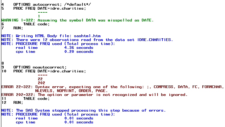
The AUTOCORRECT option is turned on by default and allows SAS to correct
syntax with small mistakes like a misspelled keyword. In the first example below,
the DATA keyword is misspelled to DATE. When the option is invoked, you will see
that in the Log (shown below), SAS issues a warning it assumed that the keyword
was misspelled and continues executing the procedure. However, in the second example where
the automatic correction option is turned off, SAS issues an error and stops
executing the procedure.
*autocorrect option;
OPTIONS AUTOCORRECT; /*default*/
PROC FREQ DATE=idre.charities;
TABLE code;
RUN;

OPTIONS NOAUTOCORRECT;
PROC FREQ DATE=idre.charities;
TABLE code;
RUN;
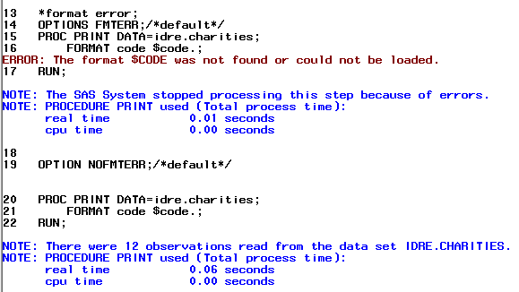
The FMTERR option controls whether SAS will issue a warning for incorrect
formats being used for variables. In this case, the default is for SAS is
to error and stop processing the executed procedure. In the first example, the
default option is invoked and as you can see below SAS issues a warning that the
format used could not be found. However, in the second example where we tell SAS
to not issue an error (NOFMTERR), SAS ignores the incorrectly used format and
will the execute the command without the format.
*format error;
OPTIONS FMTERR;/*default*/
PROC PRINT DATA=idre.charities;
FORMAT code $code.;
RUN;

OPTION NOFMTERR;
PROC PRINT DATA=idre.charities;
FORMAT code $code.;
RUN;
2.0 Diagnosing and Correcting Syntax Errors
A main issues with learning a new programming language is the ability to
identify and address coding errors. There are several ways that SAS will notify
you of syntax errors.
2.1 Color-Coded Syntax.
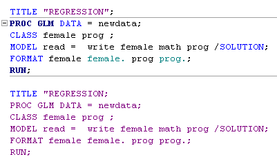
When executing code in SAS in the Enhanced
Editor you will notice some color coding. Color coding program components will
help you more easily diagnose syntax errors, and when you first start with SAS
you will make many mistakes. Take a look at the example syntax below copied from
the Enhanced Editor window. Here you will see 5 different colors
automatically generated by SAS. For example you will see that keywords like
DATA, CLASS, MODEL are all highlighted in blue. If you use the wrong keyword
with a procedure, the keyword will often remain black like the variable names because
SAS does not recognize it. Options like SOLUTION are also considered keywords. As
we will discuss later, the way to indicate a format is to put a period at then
end and, once you do this, it will turn green. Anything in quotation marks turns red.
In the second set of code, you will see that we are missing an end quote,
thus all of the syntax is red. Thus we would know to correct the missing double
quote.
2.2 Log File
The log file will also let you know when you have syntax errors. Below is an
example using PROC MEANS:

In the syntax shown, we are attempting to run the MEANS
procedure with a couple options. We have added “average” and “min” options to
our statement to indicate that we only want to the average and the minimum
values for salary. As
we described in the previous section, options should be colored in blue and in
this example “average” remains black indicating the SAS is not recognizing it as
a keyword.
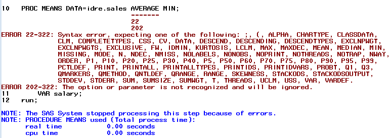
Below we see what happens when we attempt to execute the syntax as written.
An error appears in the log file indicating that the keyword “average” was not a
recognized option. Additionally, in this instance, SAS provides a list of
alternate options you may have wanted. If you look carefully, you will see that
“mean” is one of them. If we replace the unrecognized keyword “average” with
“mean” the procedure will execute as expected.
3.0 Data Step vs. Proc Step
SAS programs are comprised of two distinct steps: data steps and proc steps. Data steps are
written by you, while procedures are pre-written programs that are built-in. In
general, Data steps are used to read, modify and create data files and always begin with
a “DATA” statement. You saw an example of a data step in section 1.2.
From a statistical standpoint a Proc step is typically used to analyze a dataset
in SAS without making changes to the data. There are exceptions to this.
Proc steps always start with the familiar “PROC” statement. You have
seen several examples of Proc steps in the preceding sections including PROC
PRINT, PROC MEANS, and PROC FREQ. Each procedure enables us to analyze and
process that data in specific way.
In the following sections we will demonstrate how to use these two types of
steps.
4.0 Manipulating Datasets
4.1 Operators
An operator in SAS is a symbol representing a comparison, logical operation or
mathematical function.
4.1.1 Comparison Operator
These are operators that compare a variable with some specified value or
another variable. They are typically represented as symbols such as =, <, > but
also have mnemonic equivalents like EQ, LT, or GT, respectively. The operators
can used within a data or proc step depending on your needs.
One of the simplest ways to use a comparison operator is in a WHERE
statement. In the “sales” data file, we have information on sales associates from Australia
(AU) and the United States (US). If we only wanted to output records for
Australian sales associates we could use the = or eq operator. Since the variable
country contains character information not numeric, we need to put
single quotes around ‘AU’.
PROC PRINT DATA=idre.sales;
WHERE Country='AU';
RUN;
The IN operator can be used if you are trying to specify a
list or range of values, as demonstrated below.
PROC PRINT DATA=idre.sales;
WHERE Country IN ('AU', 'US');
RUN;
We also can specify SAS to output only certain ranges of values for numeric variables.
In the first example below we ask SAS to output salary values that are less than (<)
$30,000. In the second example, we output salary values greater than or equal to (ge) $30,000.
PROC PRINT DATA=idre.sales;
WHERE Salary<30000;
RUN;
PROC PRINT DATA=idre.sales;
WHERE Salary ge 30000;
RUN;
One limitation of using a WHERE statement is that more than 1
can not be used simultaneously, except in special cases. If you attempt
to submit the following syntax, SAS will issue a note in the Log stating “WHERE
clause has been replaced.” It will then execute the following syntax
omitting the first WHERE statement. However, in the next section we will
demonstrate how to combine comparison operators with logical operators to
achieve the desired output.
PROC PRINT DATA=idre.sales;
WHERE Country='AU';
WHERE Salary<30000;
RUN;
For more example checkout
SAS
9.4 Help and Documentation page on comparison
operators.
4.1.2 Logical Operators
The logical or Boolean operators include AND, OR,
& NOT. They are often used to link a series of comparisons.
Just like the comparison operators, these can be written as either symbols or
mnemonics. Below is table showing the each symbol and it’s mnemonic alternative.
| Symbol | Mnemonic |
| ^ ~ |
NOT |
| & | AND |
| | | OR |
In the previous section we learned that we cannot use two WHERE
statements, but we can use the AND operator to combine the information
contained in those two statements to achieve the desired result.
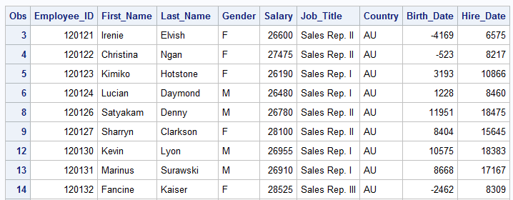
Below we use AND to output observations representing
Australian sales associates that make less than $30,000 a year. Both the symbol
and mnemonic are used and they give the same result.
PROC PRINT DATA=idre.sales;
WHERE Country='AU' AND Salary<30000;
RUN;

PROC PRINT data=idre.sales;
WHERE Country='AU' & Salary<30000;
RUN;
As with comparison operators you can also combine AND, OR,
& NOT with the IN operator. In the example
below the variable job_title includes seven different job
types. We want to obtain frequencies of all of them except for two, Sales Manager and Sales Rep
IV. So we use the NOT combined with IN since
we have more then one value we are trying to exclude.
PROC FREQ DATA=idre.sales;
TABLES Job_Title;
WHERE Job_Title NOT IN ('Sales Manager','Sales Rep. IV');
RUN;
For more example checkout
SAS
9.4 Help and Documentation page on logical
operators.
4.1.3 Where Operators
We have just covered several examples using the
comparison and logical operators.
However, SAS does include a set of special operators that can be used
only in WHERE expressions. Some of these have similar functions
to comparison operators.
|
|
|
|
|
Between-And |
Allows for an inclusive range |
Both |
|
Contains |
Includes a character string or substring |
Character Only |
|
Is Null or Is Missing |
Identifies missing values |
Both |
|
Like |
Matches a pattern |
Character Only |
|
=* |
Sounds-like |
Character Only |
|
Same-And or Also |
Augments an existing WHERE clause without have to |
Both |
For example, here are three ways of specifying that we want SAS to output all sales
associate records with salaries that range from $28,000 to $30,000. As in any
good programming language, there are always multiple ways of doing the same
thing.
* We can use only comparison operators;
PROC PRINT DATA=idre.sales;
WHERE 28000<=Salary<=30000;
RUN;

*We can use a mix of comparison and logical operators;
PROC PRINT DATA=idre.sales;
WHERE Salary>=28000 & Salary<=30000;
RUN;

*We can use only the special WHERE operators;
PROC PRINT DATA=idre.sales;
WHERE Salary BETWEEN 28000 AND 30000;
RUN;
Earlier, we discussed that, in general, SAS does not allow you to use more
then one WHERE statement in the same data or proc step. The
exception to this are the special operators “same-and” and “also”. These will
allow you to update or augment an existing WHERE statement to
add an additional conditions. In the example below the first condition
subsets the data to Australian sales associates that make less then $26,000, and then
we add the additional clause that they must also be female.
*Using Same and;
PROC PRINT DATA=idre.sales;
WHERE Country='AU' and Salary<26000;
WHERE SAME AND Gender='F';
VAR First_Name Last_Name Gender Salary Country;
RUN;
*Using Also;
PROC PRINT DATA=idre.sales;
WHERE Country='AU' & Salary<26000;
WHERE ALSO Gender='F';
VAR First_Name Last_Name Gender Salary Country;
RUN;
Now while some of these special operators are fairly self-explanatory like
“Is Null” some may be less so, such as “=*” and “Like”. These operators can be
helpful for identifying issues such as misspelled information, incorrectly
entered information, or identifying related names or titles that vary. For
example, below is a dataset called “shoes_eclipse” that includes several different
product names:
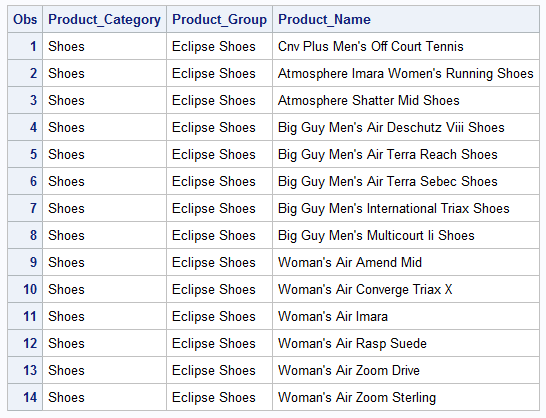
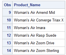
Let’s suppose we are interested in identifying product names that include the
word “Woman’s”. How could we do that? The “Like” operator could help us do this. It works by comparing character values to some given pattern.
It requires two special characters, a percent (%) sign and an underscore (_).
The percent denotes that any number of characters may occupy a position. However,
the underscore specifies that only one character may occupy a position. If we
are only interested in products that start with “Woman’s”, then we don’t care how
many spaces come after “Woman’s”:
PROC PRINT DATA=idre.shoes_eclipse;
VAR product_name;
WHERE product_name LIKE "Woman's %";
RUN;
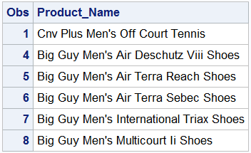
I also could ask SAS to output to me any name that includes “Men’s” any where
in the title. This would require multiple % signs b/c any
product name with “Men’s” may have character spaces before and after.
PROC PRINT DATA=idre.shoes_eclipse;
VAR product_name;
WHERE product_name LIKE "% Men's %";
RUN;
For more information check out
SAS Help and Documentation on special WHERE operators.
4.1.4 Arithmetic operators
Arithmetic operators, as you can probably tell from the name, allow you to
perform arithmetic calculations in SAS. Below is a table of the operators
and their symbols used in SAS.
| Symbol | Description |
| ** | Exponentiation |
| * | Multiplication |
| / | Division |
| + | Addition |
| – | Subtraction |
A few things to note about using these operators. First, if you are
calculating values using a variable(s) with missing data, the resulting value will also
be missing. Second, expressions are evaluated with respect to the traditional
order of operations with exponentiation taking the highest priority level, then
multiplication/division and last addition/subtraction. This ordering can be
modified by using parentheses. Third, as is the case with the other
operators we have discussed, arithmetic operators can be using on conjunction
with both logical and comparison operators.
Let’s try a few examples. Below we will use a Data step to create a new
temporary dataset called “sales_subset” from the “sales” data. This dataset will
contain only observations from Australian employees whose job title
contains the word “Rep”. So we are using a logical and special
WHERE operator. Additionally, we are creating a new variable called
“Bonus” which is calculated by multiplying “Salary” by .10.
DATA sales_subset;
SET idre.sales;
WHERE Country='AU' & Job_Title contains 'Rep';
Bonus=Salary*.10;
RUN;
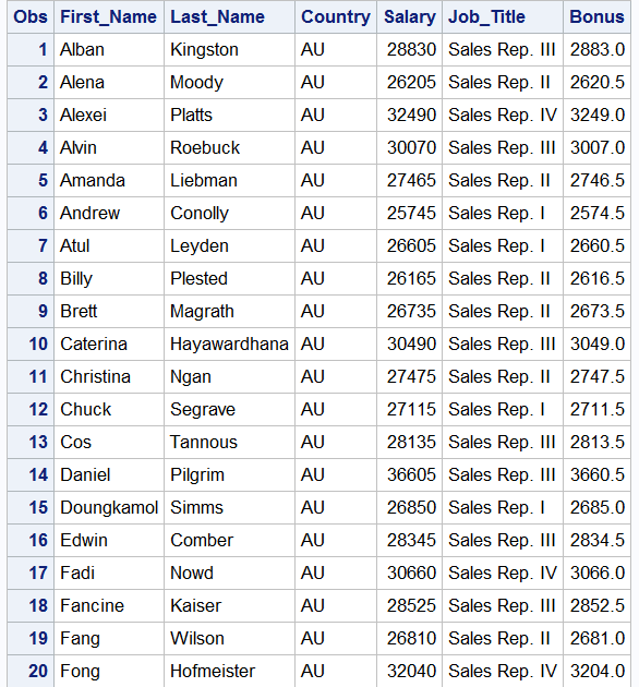
Below we output the first 20 records of our new dataset.
In this second example let’s use parentheses to change the estimation of a
compound (more then one operator)
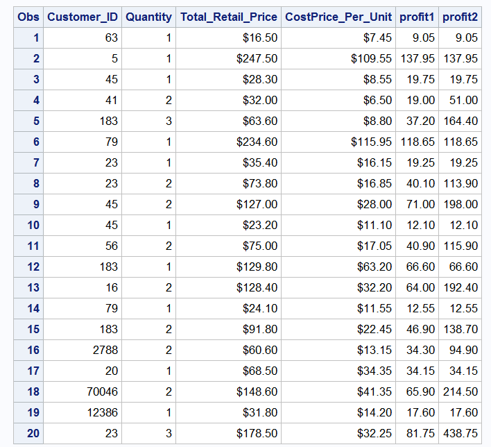
expression. We will use a Data step to create two new variables profit1 and
profit2.
DATA profit;
SET idre.order_fact;
profit1 = total_retail_price - costPrice_per_unit * quantity;
profit2 = (total_retail_price - costPrice_per_unit) * quantity;
RUN;
Let’s see how the use of parentheses has changed our values.
For more example checkout
SAS
9.4 Help and Documentation page on arithmetic
operators.
4.2 Conditional Processing
4.2.1 WHERE and
IF statements
Conditional processing in SAS allows the user to manipulate and output
portions of data instead of the whole file. In previous section you have
seen several examples of the WHERE statement.
Alternatively, SAS also allows for the use of IF statements.
Both can accomplish similar tasks; however ,while both WHERE and
IF can be used with a Data step, only WHERE is
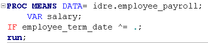
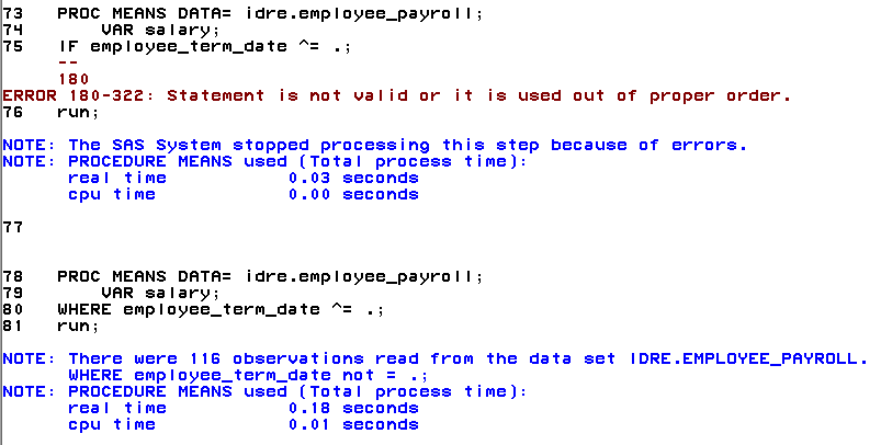
allowed in a Proc step. For example, if we add an IF statement to the
PROC MEANS
command from earlier we will see that the IF turns red.
This indicates that the syntax is incorrect.
However if you use WHERE the statement is blue.
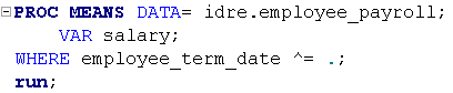
If you attempt to execute the PROC MEANS using the incorrect
IF statement SAS will produce an error but SAS will execute the
command using the WHERE statement.
Data steps will accept both WHERE and IF
statement, however only an IF can be used for assignment
statements. Below is an example of an assignment statement. Assignment in this case means we are taking observations with values for
salary that are greater than $30,000 and assigning them, using THEN
OUTPUT, to a new dataset called “highsales”.
DATA highsales ;
SET idre.sales;
IF salary GT 30000 THEN OUTPUT highsales;
RUN;
You can also combine WHERE and IF in the same Data step as demonstrated
below. We use an IF and WHERE statement to
subset the data. Can you think of equivalent ways of subsetting the data?
DATA emps;
    SET idre.sales;
WHERE Country='AU';
Bonus=Salary*.10;
IF Bonus>=3000;
RUN;
Moreover, you will notice that SAS allows you to create a variable and
use it in an IF statement in the same Data step. This is
something you can accomplish with an IF but not WHERE.
The reason for this has to do with when SAS executes conditional statements.
When using a WHERE condition SAS only selects the observations
that meets this particular condition and then continues executing
any other operations in the Data Step. This makes for more efficient
processing of data especially with large amounts of data. But in this
instance if we had used a WHERE
statement to subset the data using “Bonus”, SAS would have given us an error
saying the “Bonus” variable is not in the dataset. However, IF
conditions are not processed until the end of the Data step. Thus, SAS will
execute the WHERE statement and create “Bonus” and then assess
whether the IF condition is true.
4.2.2 If-Then statement
An If-then statement is a commonly used assignment statement that is
typically carried out within the context of Data Step. It executes a SAS
statement that fulfills a certain condition.
We will once again create a variable called “Bonus”, but assign the values
based on a certain set of conditions that are defined by an employee’s job title.
DATA comp1;
SET idre.sales;
IF Job_Title='Sales Rep. IV' THEN Bonus=1000;
IF Job_Title='Sales Manager' THEN Bonus=1500;
IF Job_Title='Senior Sales Manager' THEN Bonus=2000;
IF Job_Title='Chief Sales Officer' THEN Bonus=2500;
RUN;
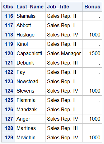
You will see in the output above, that several observations have missing
values. This is due to the fact that we did not assign values for “Bonus” for
all of the job titles.
A related statement to IF-THEN is the ELSE
statement that can be used when creating conditional statements around mutually exclusive
groups.
DATA comp2;
SET idre.sales;
IF Job_Title='Sales Rep. IV' THEN Bonus=1000;
ELSE IF Job_Title='Sales Manager' THEN Bonus=1500;
ELSE IF Job_Title='Senior Sales Manager' THEN Bonus=2000;
ELSE IF Job_Title='Chief Sales Officer' THEN Bonus=2500;
RUN;
SAS process the first IF statement and if it is not true it
moves to the next and so on. SAS continues to test the
IF-THEN
statement until it finds one that is true, which at that point it stops and will
not test the remaining conditions. Once again, this can speed up the processing of large datasets. However, as was the case
with the first
IF-THEN example, we will end up with a lot of missing values using this
syntax.
What if we had a scenario where we wanted to give all the remaining
categories, that did not fulfill the prescribed conditions, one bonus value.
We can do that using a final ELSE statement with no
IF-THEN. In the SAS code below, we add an additional ELSE
statement assigning all of the job titles a bonus value of 500.
DATA comp3;
SET idre.sales;
IF Job_Title='Sales Rep. III' or Job_Title='Sales Rep. IV' THEN Bonus=1000;
ELSE IF Job_Title='Sales Manager' THEN Bonus=1500;
ELSE IF Job_Title='Senior Sales Manager' THEN Bonus=2000;
ELSE IF Job_Title='Chief Sales Officer' THEN Bonus=2500;
ELSE Bonus=500;
RUN;
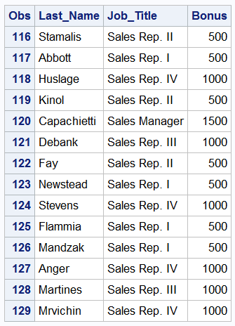
Now, we have complete data for all observations.
A second related statement to IF-THEN is the DELETE
statement. In all of the previous examples we have used the
IF-THEN statement to add information but you can also use the
IF-THEN to delete as well. Using the
IF-THEN-DELETE syntax we can specify that certain observations
fitting our condition be permanently deleted from the data. In the example
below, we delete all observations associated with three specific job titles.
DATA drop;
SET idre.sales;
IF Job_Title IN('Sales Manager', 'Senior Sales Manager', 'Chief Sales Officer') THEN DELETE;
RUN;
4.2.3 Using Do
Typically with an IF-THEN statement only one executable
statement is allowed. When an expression is true the associated statement is
executed. But what happens if you want more then one statement executed for
each expression. For example, let’s imagine that for each bonus
value, I also
want to create a variable called freq that denotes how many times a year
the sales associate can receive the bonus (e.g. once a year, twice a year). So
we might try the following code
using a logical operator.
DATA freq1;
SET idre.sales;
IF Job_Title='Sales Rep. III' or Job_Title='Sales Rep. IV' THEN Bonus=1000 & Freq = "once a year";
ELSE Bonus=500 & Freq = "twice a year";
RUN;
While this syntax appears reasonable, SAS will execute the statement
and the issue a note in the log that “Variable Freq is uninitialized”. When SAS
is unable to locate a variable in a DATA step, SAS prints this message. If you
look in the freq1 SAS dataset you will see that SAS created the variable
but sets all of it’s values to missing which is undesirable. It appears that
creating “Freq” will require a separate statement instead of just a simple “&”.
You could try this:
DATA freq2;
SET idre.sales;
IF Job_Title='Sales Rep. III' or Job_Title='Sales Rep. IV' THEN Bonus=1000;
ELSE Bonus=500;
IF Job_Title='Sales Rep. III' or Job_Title='Sales Rep. IV' THEN Freq = "once a year";
ELSE Freq = "twice a year";
RUN;
But this code could get fairly long if you have a lot of variables to create.
A better way to do this would be through the use of a DO group
which allows for multiple statements.
DATA bonus;
SET idre.sales;
IF Country='US' THEN DO;
Bonus=500;
Freq='Once a Year';
END;
ELSE DO;
Bonus=300;
Freq=’Twice a Year’;
END;
RUN;
While the syntax looks similar to a traditional IF-THEN,
there are some important differences. First, the IF expression
now ends with THEN DO. This is followed by a set of statements to
be executed. Second, each DO block ends with an END
statement. Third, instead of just ELSE we now have ELSE DO
which also has an END statement. If you are missing an
END, SAS will issue a warning in the log and fail to execute the Data step.
4.3 SAS Functions
Functions accepts arguments and then produce a particular value (numeric or
character) based on those arguments. Arguments are enclosed within parentheses
and each argument is separated by a comma. SAS has a wide array of different
functions depending on the needs of the user and can be used
in Data step. We will cover a few examples of basic mathematical
functions, common date functions, and some additional functions useful for
specific data
management tasks.
4.3.1 Arithmetic Functions
In the first example, we will use the “Oldbudget” data file to calculate
the total
and average amount budgeted for business operations over a five year period.
DATA budget;
SET idre.oldbudget;
sum1 = yr2003 + yr2004 + yr2005 + yr2006 + yr2007;
sum2 = SUM(yr2003, yr2004, yr2005, yr2006, yr2007);
sum3 = SUM( of yr2003-yr2007);

mean1 = (yr2003 + yr2004 + yr2005 + yr2006 + yr2007)/5;
mean2 = MEAN(yr2003, yr2004, yr2005, yr2006, yr2007);
mean3 = MEAN( of yr2003-yr2007);

RUN;
There are many different way of creating the sum and mean variables that we need. We
create “sum1” using an arithmetic operator to add the 5 budget amount together.
Alternatively, we can use the SUM() function, the arguments are
the variables you wish to sum together. The difference between using the
function versus manually adding together each variable is the treatment of
missing. When we add items using “+”, a case with missing values on any of the
variables listed will have a missing value for the resulting variable. If we use
the SUM() function, any missing values will be treated
as though they were zero, and the new variable will be equal to missing only if
all of the variables listed are missing. Which method is most appropriate
depends on the situation and what you are trying to achieve. Last, if you have
a lot of variables to be summed you can specify a SAS variable list. This syntax
works since the variable being specified are consecutive in the data. Check the
SAS documentation page on
SAS variable lists on how to use this shortcut in other circumstances. We
also use similar syntax to demonstrate how to estimate the average or mean
budget variables.
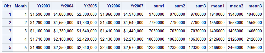
All the values produced for “sum1-sum3” and “mean1-mean3” are the same since
we do not have any missing data. SAS has a number of additional
mathematical functions including absolute value, maximum, minimum and square
root that can be used in a similar manner.
4.3.2 Date Functions
One of the more challenging data types to deal with in any data analysis
package are date values. Thankfully, SAS has some built-in functions that
can assist users with managing this data type. SAS stores date information as numeric
values representing the number days before or after Jan 1, 1960. SAS can
also recognize 2 or 4 digit year values. We will use the “Sales” dataset which
includes information on date of birth and hiring data for each employee to
demonstrate some date functions.
DATA comp;
SET idre.sales;
Hire_Month=MONTH(Hire_Date);
Birth_Day = WEEKDAY(Birth_date);
Day_Dif = DATDIF(Birth_date,Hire_Date, 'actual');
Month_dif= INTCK('years',Birth_date,Hire_Date);
Bonus_1 = INTNX('month', Hire_Date, 6);
RUN;
The MONTH function pulls the month from “Hire_date” and put’s
it in a variable called “Hire_month”. The WEEKDAY function
figures out what day of the week (1-7) the date would have fallen on and outputs
this.
DATDIF calculates the difference in days between two dates
given in the first two arguments. The third argument specifies the method for
calculating the days. In this example we specify we want the ‘actual’ number of
days, but we could choose other methods of calculation such assuming that each month has 30 days and that a year
always has 360 days.
INTCK counts the number of intervals between two dates, in
our example we asked SAS to output the number of years between an employees data
of birth and when they were hired which we would be equivalent to an employees
age at the time of hire.
INTNK is used to estimate calculate the variable
bonus_1. Here
we want to calculate when an employee with be eligible for their next bonus. The
arguments for this function are the unit of time, the variable representing the
start date/time and the number of increments. In our example, employees are
eligible 6 months after their hire date.
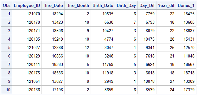
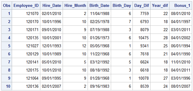
Below is the output of the first 10 observations of the “comp” dataset, with
and without date formats. As mentioned before, SAS stores date information as
numeric information in days. Thus if you do not format date with a format
statement (discussed further in the next section), it will display as just a
number.
PROC PRINT DATA=comp (OBS=10);
VAR Employee_ID Hire_date Hire_Month Birth_date Birth_Day Day_dif Month_dif Bonus_1;
*FORMAT Hire_date Birth_date Bonus_1 mmddyy10.;
RUN;
More example of SAS date function can be found on the
SAS Help and Documentation website.
4.3.3 Other Functions
SAS includes several other types of functions designed for specific types of
needs many of these functions are helpful for data management of character or
string information. For example, LENGTH tells the user the
length of a character string while COMPRESS will compress string
values and remove unwanted blanks and specific character values like dashes.
Additionally, in similar way to extracting date information like the
MONTH function, SAS has several functions including SCAN
and SUBSTR that allows you to extract words from a
phrase.
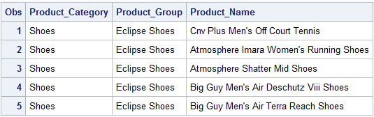
Let’s demonstrate these. Below is sample of data from a data set called
“Shoes_eclipse” where all the variables have character information. Our task of
interest is to obtain the length of product_name, compress
product_name to
remove the blanks, and create a variable the extracts the brand name
“Eclipse” from product_group.
DATA shoes;
SET idre.shoes_eclipse;
length_name = LENGTH(product_name);
comp_product = COMPRESS(product_name);
brand = SUBSTR(product_group, 1, 7);
brand2 = SCAN(product_group, 1, " ");
RUN;
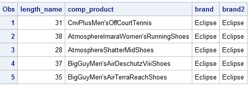
You will notice a few things about the output above. First, for the variable
length_name, if you counted the number of letters and spaces in
product_name
you would end up with the same values displayed above. Second, the
compressed version of product_name now includes no spaces. Third, both
SCAN and SUBSTR functions produced the same
output. The SUBSTR function takes 3 arguments, the name of
variable with the information you want to extract, the character position you
want to start from and then the number of character to extract. In our example
we are telling SAS that we want to extract a character string of length 7
starting at the first character position of “product group” which would be the
“E” in Eclipse. Unfortunately, this means whatever value we are extracting must
always be of the same length. What if we have product names of different
lengths. Then you might want to use the SCAN function, which work very
similar to SUBSTR except, instead of specifying the length of
the string, the last argument is a delimiter. The syntax above indicates that
the character string of interest starts at the first position and continues until
a blank/space is encountered. This function works with many types of
delimiters including < ( + & ! $ * ) ; ^ – / , % .
In the previous examples, we were extracting values from a string, but what if
we wanted to combine string variables. A useful function would be CATX.
Below we want SAS to combine the character string information in first_name
and last_name into one fullname variable. Additionally,
the function also requires the
specification of variables that includes information on the delimiter of choice.
In the first example, the delimiter is just a blank while in the second example
the delimiter is a comma.
DATA salesquiz;
SET idre.salesquiz;
sep = " ";
fullname = CATX(sep, first_name, last_name);
sep1 = ",";
fullname1 = CATX(sep1, last_name, first_name);
RUN;
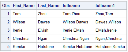
The new variables are displayed above.
A list of all SAS functions, by category, can be found
here on the SAS website.
Note: The order in
which the variables are specified in the CATX function governs the order in which
they will be combined.
4.4 Sorting, Merging and Appending
4.4.1 Sorting
The are many
instances when having your data sorted in a particular way will be helpful for
visualizing your data. Additionally, certain types of data management needs like
merging datasets or grouping observations by a particular characteristic require
sorting.
Sorting data by a single variable in SAS is the most simple. By
default SAS sorts data ascending with the smaller values first.
PROC SORT DATA=idre.sales OUT=sales; *OUT= is optional;
BY Salary;
RUN;
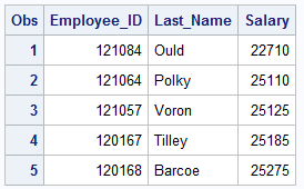
Sorting can also be done using more then one variable.
PROC SORT DATA=idre.sales OUT=sales;
BY Salary Country;
RUN;
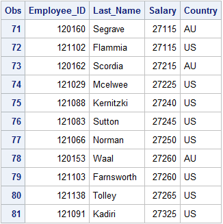
As you can see, the data is sorted in ascending order by “Salary ” first and
then when there are tied salaries from different countries, AU comes before US
alphabetically. We can change this sorting behavior flipping the ordering
of our variables and/or adding in the DESCENDING option, which reverses the
sort order for the variable that immediately follows it.
PROC SORT DATA=idre.sales OUT=sales;
BY DESCENDING Salary DESCENDING Country;
RUN;
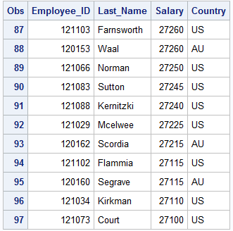
4.4.2 Merging
One data management task that requires proper sorting is merging.
Merging involves matching one observation in a dataset to one observation
(One-to-One) or multiple observations (One-to-Many) in a second dataset. In order
for this to be done properly in SAS, the datasets to be merged must be sorted by
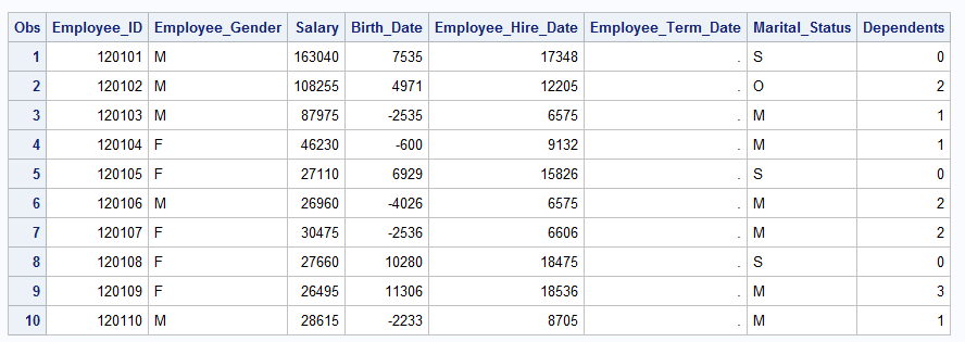
the same variable(s). In the example below, we will merge a dataset
that has employee payroll information with a second dataset with employee
addresses. Since an employee’s ID number (employee_id) is a unique identifier of each observation, we
will use this variable to match observations.
First, we need sort each dataset by employee_id.
PROC SORT DATA=idre.employee_payroll OUT=payroll;
BY Employee_ID;
RUN;
PROC SORT DATA=idre.employee_addresses OUT=addresses;
BY Employee_ID;
RUN;
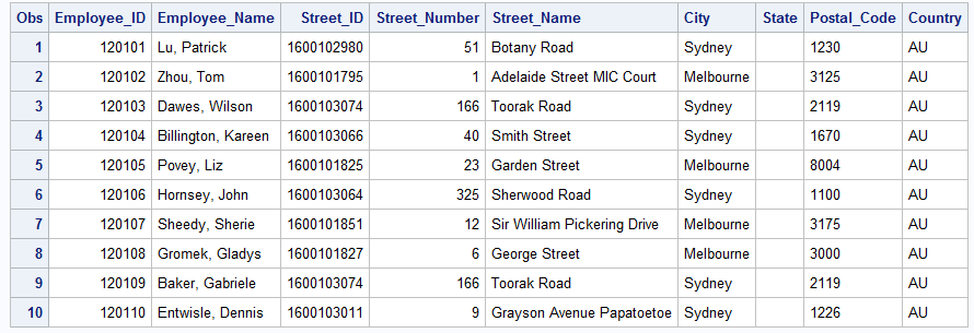
A few things to take note of. First, You will notice that datasets “addresses”
and “payroll” do not share any of the same variables except Employee_ID. In general, you do
not want to merge datasets that include variables with the same names. SAS can
only use one set of values and will arbitrarily choose the values from the last
dataset read. Thus, you should rename variables before attempting the
merge. Second, Employee_ID is unique in each
dataset, so this will be a One-to-One merge.
Merging is done in a Data step similar to what we have been executing, except
instead of the SET statement we now have a MERGE
statement. Additionally, the BY is used to tell SAS which
variable will be used to match records. The variable after the BY
statement is the same unique identifier that we just used for sorting.
DATA payadd;
MERGE payroll addresses;
BY Employee_ID;
RUN;
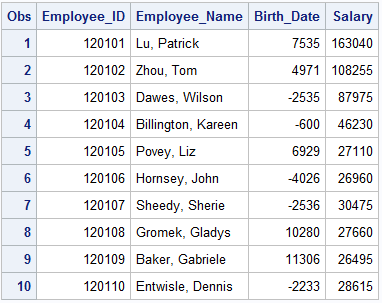
Below is a subset of variables from the newly merged data. As you can see,
Employee_Name is from the “addresses” data and
Birth_date and Salary are from the “payroll” data.
Now let’s take a look at an example of a One-to-Many merge.
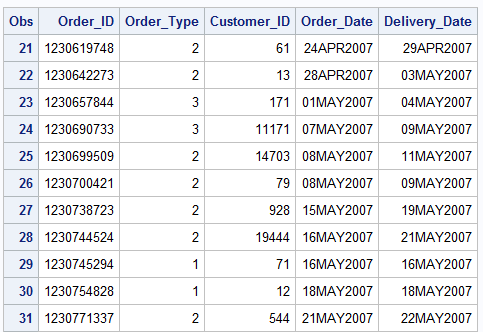
The first set of data provides information on order and delivery
dates. In the second set of data we have information
on the product or products ordered. Because more then one item can be associated
with a particular Order_ID, it is not unique in this dataset.
Thus, we will need to conduct a one to many merge where each row in our “orders”
data could be merged with multiple rows in the “order_item” data.
Again, we will
begin by sorting both sets of data by Order_ID.
PROC SORT DATA=idre.orders OUT= orders;
BY Order_id;
RUN;
PROC SORT DATA=idre.order_item OUT= order_item;
BY Order_id;
RUN;
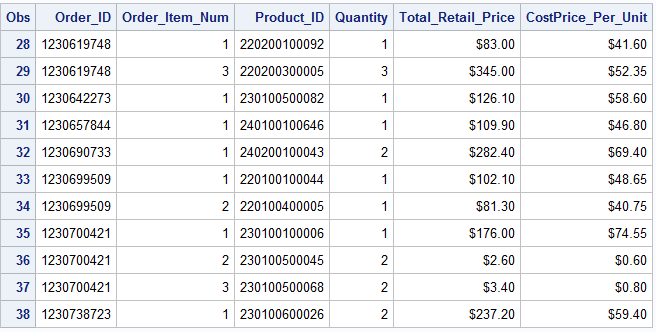
Below is our syntax to merge the two data sets. Notice we also used a
KEEP statement. This allows us to merge the data and control the
number variables present in the final merged dataset.
DATA allorders;
MERGE orders order_item;
BY Order_ID;
KEEP Order_ID Order_Item_Num Order_Type Order_Date Quantity Total_Retail_Price;
RUN;
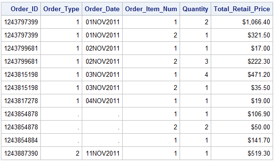
Above is a selected portion of the merged data. SAS executed the merge without
an error but it appears that we have some missing data as a result. The two
variables that have missing information were both from the “orders” data.
This is an indication that we perhaps have some non-matches. If we go back and
look at the “orders” data we would see that there is no information for the
order identifier “1243854878” but there is information in “order_item”, thus
when you merge the datasets together all the variables from “orders” will have
missing values for this particular order. There are a couple ways you can deal
with this issue. First, you can leave the data as is with missing information
for non-matches. Alternatively, you can choose to control the observations
output to the new merged data set by using the IN option on the
MERGE statement. The IN option a creates
variable indicating which dataset(s) contributed to forming the observation in
the final merge dataset. It is a temporary variable used in the merging process
that is given a 0 value if did not provide information or a 1 if it did.
We could then use this variable to select observations in the newly merged data
that come from one dataset or both. Let’s take a look at how we could
apply this option in our previous merge.
DATA allorders2;
MERGE orders (in=a)
      order_item (in=b);
BY Order_ID;
KEEP Order_ID Order_Item_Num Order_Type Order_Date Quantity Total_Retail_Price;
IF a;
RUN;
Using the IN option with an IF statement
selects observations to be matched by order_ID that are present
in “orders”. If you have a value for order_ID that is in
“order_item” but not “orders” then it will not be used to construct
observations
for the “allorders2” data set. Note: Using IF=a is equivalent to saying IF a=1. Thus, you will not end up with any missing values.
Now, one thing you generally want to avoid is many-to-many merges. When neither dataset
has a unique identifier that will allow for proper matching
of records the result is a somewhat unpredictable and often undesirable
assorting of observations.
4.4.3 Appending
Appending or concatenating observations is the process of adding rows or
observations to a dataset as opposed to merging which adds variables. This can
also be accomplished using a Data step. SAS will stack the columns to together by
matching the names across datasets.
We will append three datasets that include information on orders from 3
consecutive months (July-September) in 2011. Below is snapshot of the
first two records from each of the datasets to be appended.
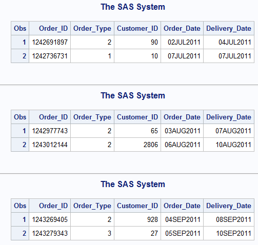
The syntax to conduct the append is quite simple. All you have to do is
list the datasets to be appended on the SET statement line. The
ordering and the number of datasets does not matter.
DATA mnth7_8_9_2011 ;
SET idre.mnth7_2011 idre.mnth8_2011 idre.mnth9_2011;
RUN;
A portion of the newly appended dataset is below.
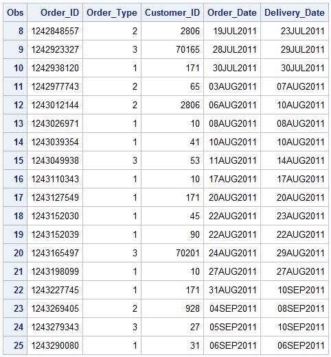
Now you can see that all 3 datasets has been appended or “stacked” together.
This example worked perfectly because the three datasets shared the exact same
variables. But what happens when you append the datasets that do not contain the
same variables?
Take a look back at our “shoe” data. Below we have two sets of data, one for
Eclipse shoes and one for Tracker Shoes. You will notice they share all the same
variables except two, product_id and supplier_name.
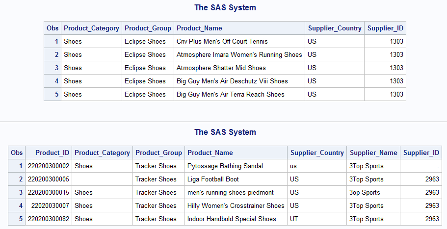
What will happen when we attempt to append the data?
DATA shoes;
SET idre.shoes_eclipse idre.shoes_tracker;
RUN;
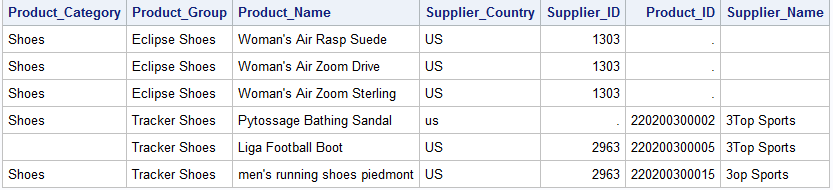
The append still executes without error. However, in the new “shoes” data we created, all the records from the Eclipse dataset
will be missing on the variables that were only in the Tracker dataset.
5.0 Modifying SAS Output
5.1 Titles and Footnotes
As you have probably already noticed, SAS provides a lot of output from many
of it’s procedures. As a researcher it is important to know how to
manipulate and change your output to convey important information to your
audience. One of the procedures we have been using to obtain output from our
various Data steps is PROC PRINT. We will begin by
exploring some ways of enhancing the output from this procedure.
Whenever you are presenting tables of information, the first item most people
look for is a title. This is easily implemented with a TITLE
statement in SAS. Additionally, it is also possible to add multiple titles to output
in SAS as well as footnotes by just adding a numeric suffix to the statement
indicating the desired ordering. SAS allows for up to 10 different titles and/or
footnotes.
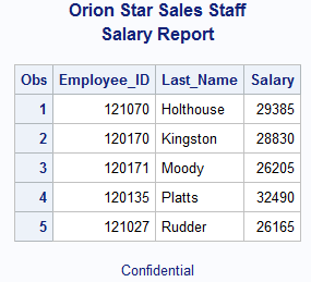
TITLE1 'Orion Star Sales Staff';
TITLE2 'Salary Report';
FOOTNOTE1 'Confidential';

PROC PRINT DATA=idre.sales (OBS=5);
VAR Employee_ID
Last_Name Salary;
RUN;
5.2 Label Options
Additionally, you may also find it useful to label your variables for added
readability. You can do this with the LABEL statement. You will notice that some of the variable labels are longer than others. When
you only have three variables it may not seem important, but if you have to label
10 variables, available space in a table may need to be a consideration. One way to deal with this
is to use the SPLIT option on the PROC PRINT
line. This allows the user to control the display of the title so that instead of
the label being one line, you can split it into two lines.
PROC PRINT DATA=idre.sales (OBS=5) SPLIT='*';
VAR Employee_ID Last_Name Salary;
LABEL Employee_ID = 'Sales ID'
      Last_Name = 'Last*Name'
      Salary = 'Annual*Salary';
RUN;
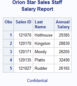
The variable names have been replaced with labels. Note that we did not have to resubmit the TITLE and FOOTNOTE statements. These are considered global statements and remain in effect until you cancel them or you end your SAS session. To cancel these you must issue a blank statement for each:
TITLE;
FOOTNOTE;
5.3 Formats
Beyond just labeling variables, you may also want to properly label the
values of those variables. This is carried out in SAS using a FORMAT
statement. Formatting values changes the appearance of those values in output but the underlying values does NOT change.
SAS has pre-defined formats for certain types of variables like dates and allows users to create their own formats for specific situations. Earlier we saw some examples of pre-defined formats when we covered date
functions. Here, we will focus on how to create and apply user-defined
formats.
In SAS, the PROC FORMAT procedure is used to define formats.
For example, take a look at the syntax below:
PROC FORMAT;
VALUE $ctryfmt     'AU'='Australia'
                   'US'='United States'
                    other ='Miscoded';

VALUE tiers         0-49999='Tier 1'
                    50000-99999='Tier 2'
                    100000-250000='Tier 3';
RUN;
Each format is defined after a VALUE statement. The name you
choose is up to you. Notice that character formats must be defined with a
“$” in front of them. You then provide a value label for each level or range of
values. The first format we are creating is to label the countries will their
full names instead of abbreviations. VALUE statements can also use keywords.
In this example
other specifies that any values other then AU or US will
be labeled as “Miscoded’. For numeric formats, you can label a single
value or a range of values. Once the formats are created we can apply them to
the variables of interest.
In both Data steps and Proc steps, SAS distinguishes formats from
variables by ending them in a period which then turns the text green.
PROC PRINT DATA=idre.sales (OBS=5);
VAR Employee_ID Salary Country Birth_Date Hire_Date;
FORMAT Salary tiers. Birth_Date Hire_Date monyy7. Country $ctryfmt.;
RUN;
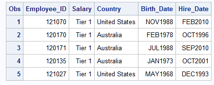
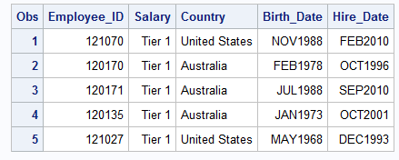
Above you can see the appearance of the table with unformatted values to the
one with formatted values. If you only want to use the formatted values for
certain procedures in SAS, then you can just add a format statement as we did
above. If you want these formats to be permanently applied to a variable, then
you can use the same format statement in a Data Step.
5.4 Output Delivery System (ODS) Basics
Besides customizing the SAS default output, you may want to output results to
different file types. By default SAS 9.4 output
results as HTML and this is what you see in the “Results Viewer” window.
If you would like to change this behavior, you will need to use the Output
Delivery System (ODS) statement. This will allow for output in several
different formats including listing/text, rtf, pdf and .xls.
ODS statements are also global statements are in effect until closed. The statement comes before running the procedure. Once the procedure(s) is
executed, you will then close the ODS statement. The basic syntax is shown
below:
ODS PDF FILE="&pathexample.pdf";
ODS RTF FILE="&pathexample.rtf";

PROC FREQ DATA=<data>;
TABLES <variable>;
RUN;

ODS PDF CLOSE;
ODS RTF CLOSE;
In this case, the output from the PROC FREQ will be saved to
a pdf file and a rtf file. You must also specify the path or location where you
want these documents saved. Once complete you should then close the output
destination otherwise SAS will keep sending your results to these documents.
Before SAS 9.3 the default output destination was listing. You can see
the results from the PROC FREQ in the Output window and see a
new icon in the Results tab.
ODS LISTING;
PROC FREQ DATA=idre.sales;
TABLES gender;
RUN;
ODS LISTING CLOSE;
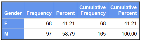
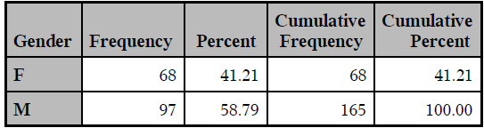
As a user, you can also customize the style or look of the output when
selecting either a html, pds or rtf destination. This ability is often useful
when formatting results for presentations or publications. Below are some
examples of the different options available in SAS:
ODS HTML FILE="C:myreport.html" STYLE=sasweb;
PROC FREQ DATA=idre.sales;
TABLES gender;
RUN;
ODS HTML CLOSE;
ODS PDF FILE="C:myreport.pdf" STYLE=printer; /*Default*/
ODS PDF FILE="C:myreport1.pdf" STYLE=journal;
PROC FREQ DATA=idre.sales;
TABLES gender;
RUN;
ODS PDF CLOSE;
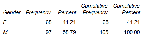
Just to be safe we will go ahead and close all of the open destinations.
However, be mindful that this will also close the html default, so you will
need to reissue the global statement turning it back on. Otherwise the next time
you issue a procedure that generates output, SAS will issue the warning “No
output destination active”.
ODS _ALL_ CLOSE;
ODS HTML;
6.0 Special Issues
6.1 Dealing with Duplicates
An issue that comes up a lot in data management is how to handle duplicates.
There are several ways in SAS to identify duplicate records.
One way is to use some of the options available to us with the PROC
FREQ procedure. In the “nonsales” data file, we should have 235 unique
employee identification numbers. We can use the ORDER=FREQ
option to determine if this is true. This option displays the frequency of each
unique identification number in descending order.
PROC FREQ DATA=idre.nonsales ORDER=FREQ;
TABLES Employee_ID;
RUN;
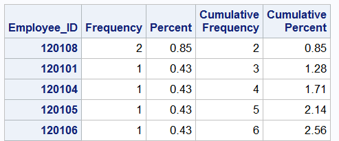
Above you can see that the employee ID #120108 has two records
associated with it, indicating that we have a duplicate problem. Another useful option
is NLEVELS, which displays the number of distinct values for
each variable.
PROC FREQ DATA=idre.nonsales NLEVELS;
TABLES Employee_ID /NOPRINT;
RUN;

There are 235 unique employees in the “nonsales” data but only 234 unique
levels, meaning that one employee ID# is duplicated.
Once the presence of duplicate ID numbers has been confirmed, you will most
likely want to examine them to determine if they are indeed duplicate records or
if the employee ID number is incorrect. In our dataset only one ID is duplicated
making assessment fairly easy. However, what do you do when several ID’s or
records are duplicated? Let’s separate the records with unique ID’s from
the duplicates using an IF statement.
PROC SORT DATA=idre.nonsales OUT=ids2;
BY employee_id;
RUN;

DATA dupes nodupes;
SET ids2;
BY employee_id;
IF NOT (FIRST.employee_id and LAST.employee_id) THEN OUTPUT dupes;
ELSE OUTPUT nodupes;
RUN;
Above we are using the keywords FIRST. and LAST.
These keywords identify the first and last record in the grouping
variable indicated after the BY statement. When an employee ID is unique, the
first and last record will be the same row. Thus our code outputs employee
ID’s where the first and last records are not the same, to a dataset called
“dupes”, and all the other unique records are put in dataset called “nodupes”.
“Dupes” or duplicated employee ID numbers:

“NoDupes” or unique employee ID numbers.

6.2 Identifying Outliers
Another issue that comes up a lot in dealing with data is outliers. The simplest way in SAS to identify outliers in to use the UNIVARIATE
procedure.
By default, the UNIVARIATE
procedure outputs the 5 highest and lowest extreme observations. Let’s
examine outliers for product prices in the “price_new” dataset.
PROC UNIVARIATE DATA=idre.price_new;
VAR unit_cost_price;
RUN;
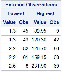
You can override this default by specifying the option NEXTROBS = on the
procedure line and indicate the number of outliers to display. You can specify
any number between 0 and half of the total observations. You will also notice
that along with the extreme values, SAS also provides an observation or row
number that corresponds to this value. Additionally, you can also use the ID
statement to identify observations. This statement specifies one or more
variables to be included in the outliers table. Let’s try adding the product
identifier Product_ID to each of our extreme values.
PROC UNIVARIATE DATA=idre.price_new NEXTROBS=3;
VAR unit_cost_price;
ID Product_ID;
RUN;
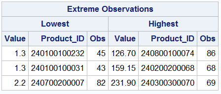
Now each extreme value is associated with it’s ID number.
7.0 Wrapping things up
As we stated in the beginning, SAS is a very flexible programs with great
features for data management.
This seminar only scratches the surface on describing all of the programming
options available to users.
For more information on the topics discussed here please explore our
website.
Additionally, SAS has a host of courses designed to improve your programming
skills aimed at users of all levels.