1. Introduction
Survival analysis models factors that influence the time to an event. Ordinary least squares regression methods fall short because the time to event is typically not normally distributed, and the model cannot handle censoring, very common in survival data, without modification. Nonparametric methods provide simple and quick looks at the survival experience, and the Cox proportional hazards regression model remains the dominant analysis method. This seminar introduces procedures and outlines the coding needed in SAS to model survival data through both of these methods, as well as many techniques to evaluate and possibly improve the model. Particular emphasis is given to proc lifetest for nonparametric estimation, and proc phreg for Cox regression and model evaluation.
Note: A number of sub-sections are titled Background. These provide some statistical background for survival analysis for the interested reader (and for the author of the seminar!). Provided the reader has some background in survival analysis, these sections are not necessary to understand how to run survival analysis in SAS. These may be either removed or expanded in the future.
Note: The terms event and failure are used interchangeably in this seminar, as are time to event and failure time.
1.1 Sample dataset
Click here to download the dataset used in this seminar.
In this seminar we will be analyzing the data of 500 subjects of the Worcester Heart Attack Study (referred to henceforth as WHAS500, distributed with Hosmer & Lemeshow(2008)). This study examined several factors, such as age, gender and BMI, that may influence survival time after heart attack. Follow up time for all participants begins at the time of hospital admission after heart attack and ends with death or loss to follow up (censoring). The variables used in the present seminar are:
- lenfol: length of followup, terminated either by death or censoring. The outcome in this study.
- fstat: the censoring variable, loss to followup=0, death=1
- age: age at hospitalization
- bmi: body mass index
- hr: initial heart rate
- gender: males=0, females=1
The data in the WHAS500 are subject to right-censoring only. That is, for some subjects we do not know when they died after heart attack, but we do know at least how many days they survived.
Before we dive into survival analysis, we will create and apply a format to the gender variable that will be used later in the seminar.
proc format library=mylib;
value gender
	  0 = "Male"
	  1 = "Female";
run;

data whas500;
set whas500;
format gender gender.;
run;
1.2. Background: Important distributions in survival analysis
Understanding the mechanics behind survival analysis is aided by facility with the distributions used, which can be derived from the probability density function and cumulative density functions of survival times.
1.2.1. Background: The probability density function, \(f(t)\)
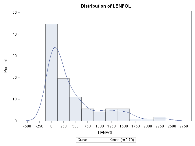
Imagine we have a random variable, \(Time\), which records survival times. The function that describes likelihood of observing \(Time\) at time \(t\) relative to all other survival times is known as the probability density function (pdf), or \(f(t)\). Integrating the pdf over a range of survival times gives the probability of observing a survival time within that interval. For example, if the survival times were known to be exponentially distributed, then the probability of observing a survival time within the interval \([a,b]\) is \(Pr(a\le Time\le b)= \int_a^bf(t)dt=\int_a^b\lambda e^{-\lambda t}dt\), where \(\lambda\) is the rate parameter of the exponential distribution and is equal to the reciprocal of the mean survival time. Most of the time we will not know a priori the distribution generating our observed survival times, but we can get and idea of what it looks like using nonparametric methods in SAS with proc univariate. Here we see the estimated pdf of survival times in the whas500 set, from which all censored observations were removed to aid presentation and explanation.
proc univariate data = whas500(where=(fstat=1));
var lenfol;
histogram lenfol / kernel;
run;
In the graph above we see the correspondence between pdfs and histograms. Density functions are essentially histograms comprised of bins of vanishingly small widths. Nevertheless, in both we can see that in these data, shorter survival times are more probable, indicating that the risk of heart attack is strong initially and tapers off as time passes. (Technically, because there are no times less than 0, there should be no graph to the left of LENFOL=0)
.
1.2.2. Background: The cumulative distribution function, \(F(T)\)
The cumulative distribution function (cdf), \(F(t)\), describes the probability of observing \(Time\) less than or equal to some time \(t\), or \(Pr(Time ≤ t)\). Above we described that integrating the pdf over some range yields the probability of observing \(Time\) in that range. Thus, we define the cumulative distribution function as:
\[F(t) = \int_0^tf(t)dt\]
As an example, we can use the cdf to determine the probability of observing a survival time of up to 100 days. The above relationship between the cdf and pdf also implies:
\[f(t) = \frac{dF(t)}{dt}\]
In SAS, we can graph an estimate of the cdf using proc univariate.
proc univariate data = whas500(where=(fstat=1));
var lenfol;
cdfplot lenfol;
run;
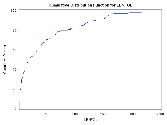
In the graph above we can see that the probability of surviving 200 days or fewer is near 50%. Thus, by 200 days, a patient has accumulated quite a bit of risk, which accumulates more slowly after this point. In intervals where event times are more probable (here the beginning intervals), the cdf will increase faster.
1.2.3. Background: The Survival function, S(t)
A simple transformation of the cumulative distribution function produces the survival function, \(S(t)\):
\[S(t) = 1 – F(T)\]
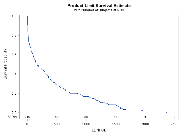
The survivor function, \(S(t)\), describes the probability of surviving past time \(t\), or \(Pr(Time > t)\). If we were to plot the estimate of \(S(t)\), we would see that it is a reflection of F(t) (about y=0 and shifted up by 1). Here we use proc lifetest to graph \(S(t)\).
proc lifetest data=whas500(where=(fstat=1)) plots=survival(atrisk);
time lenfol*fstat(0);
run;
It appears the probability of surviving beyond 1000 days is a little less than 0.2, which is confirmed by the cdf above, where we see that the probability of surviving 1000 days or fewer is a little more than 0.8.
1.2.4. Background: The hazard function, \(h(t)\)
The primary focus of survival analysis is typically to model the hazard rate, which has the following relationship with the \(f(t)\) and \(S(t)\):
\[h(t)=\frac{f(t)}{S(t)}\]
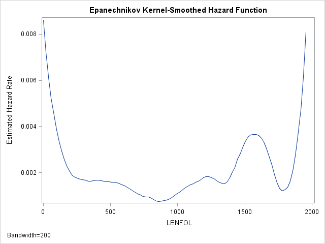
The hazard function, then, describes the relative likelihood of the event occurring at time \(t\) (\(f(t)\)), conditional on the subject’s survival up to that time \(t\) (\(S(t)\)). The hazard rate thus describes the instantaneous rate of failure at time \(t\) and ignores the accumulation of hazard up to time \(t\) (unlike \(F(t\)) and \(S(t)\)). We can estimate the hazard function is SAS as well using proc lifetest:
proc lifetest data=whas500(where=(fstat=1)) plots=hazard(bw=200);
time lenfol*fstat(0);
run;
As we have seen before, the hazard appears to be greatest at the beginning of follow-up time and then rapidly declines and finally levels off. Indeed the hazard rate right at the beginning is more than 4 times larger than the hazard 200 days later. Thus, at the beginning of the study, we would expect around 0.008 failures per day, while 200 days later, for those who survived we would expect 0.002 failures per day.
1.2.5. Background: The cumulative hazard function
Also useful to understand is the cumulative hazard function, which as the name implies, cumulates hazards over time. It is calculated by integrating the hazard function over an interval of time:
\[H(t) = \int_0^th(u)du\]
Let us again think of the hazard function, \(h(t)\), as the rate at which failures occur at time \(t\). Let us further suppose, for illustrative purposes, that the hazard rate stays constant at \(\frac{x}{t}\) (\(x\) number of failures per unit time \(t\)) over the interval \([0,t]\). Summing over the entire interval, then, we would expect to observe \(x\) failures, as \(\frac{x}{t}t = x\), (assuming repeated failures are possible, such that failing does not remove one from observation). One interpretation of the cumulative hazard function is thus the expected number of failures over time interval \([0,t]\). It is not at all necessary that the hazard function stay constant for the above interpretation of the cumulative hazard function to hold, but for illustrative purposes it is easier to calculate the expected number of failures since integration is not needed. Expressing the above relationship as \(\frac{d}{dt}H(t) = h(t)\), we see that the hazard function describes the rate at which hazards are accumulated over time.
Using the equations, \(h(t)=\frac{f(t)}{S(t)}\) and \(f(t)=-\frac{dS}{dt}\), we can derive the following relationships between the cumulative hazard function and the other survival functions:
\[S(t) = exp(-H(t))\] \[F(t) = 1 – exp(-H(t))\] \[f(t) = h(t)exp(-H(t))\]
From these equations we can see that the cumulative hazard function \(H(t)\) and the survival function \(S(t)\) have a simple monotonic relationship, such that when the Survival function is at its maximum at the beginning of analysis time, the cumulative hazard function is at its minimum. As time progresses, the Survival function proceeds towards it minimum, while the cumulative hazard function proceeds to its maximum. From these equations we can also see that we would expect the pdf, \(f(t)\), to be high when \(h(t)\) the hazard rate is high (the beginning, in this study) and when the cumulative hazard \(H(t)\) is low (the beginning, for all studies). In other words, we would expect to find a lot of failure times in a given time interval if 1) the hazard rate is high and 2) there are still a lot of subjects at-risk.
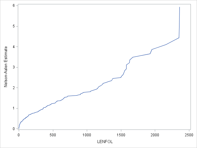
We can estimate the cumulative hazard function using proc lifetest, the results of which we send to proc sgplot for plotting. We see a sharper rise in the cumulative hazard right at the beginning of analysis time, reflecting the larger hazard rate during this period.
ods output ProductLimitEstimates = ple;
proc lifetest data=whas500(where=(fstat=1))  nelson outs=outwhas500;
time lenfol*fstat(0);
run;
proc sgplot data = ple;
series x = lenfol y = CumHaz;
run;
2. Data preparation and exploration
2.1. Structure of the data
This seminar covers both proc lifetest and proc phreg, and data can be structured in one of 2 ways for survival analysis. First, there may be one row of data per subject, with one outcome variable representing the time to event, one variable that codes for whether the event occurred or not (censored), and explanatory variables of interest, each with fixed values across follow up time. Both proc lifetest and proc phreg will accept data structured this way. The WHAS500 data are stuctured this way. Notice there is one row per subject, with one variable coding the time to event, lenfol:
| Obs | ID | LENFOL | FSTAT | AGE | BMI | HR | GENDER |
|---|---|---|---|---|---|---|---|
| 1 | 1 | 2178 | 0 | 83 | 25.5405 | 89 | Male |
| 2 | 2 | 2172 | 0 | 49 | 24.0240 | 84 | Male |
| 3 | 3 | 2190 | 0 | 70 | 22.1429 | 83 | Female |
| 4 | 4 | 297 | 1 | 70 | 26.6319 | 65 | Male |
| 5 | 5 | 2131 | 0 | 70 | 24.4125 | 63 | Male |
A second way to structure the data that only proc phreg accepts is the “counting process” style of input that allows multiple rows of data per subject. For each subject, the entirety of follow up time is partitioned into intervals, each defined by a “start” and “stop” time. Covariates are permitted to change value between intervals. Additionally, another variable counts the number of events occurring in each interval (either 0 or 1 in Cox regression, same as the censoring variable). As an example, imagine subject 1 in the table above, who died at 2,178 days, was in a treatment group of interest for the first 100 days after hospital admission. This subject could be represented by 2 rows like so:
| Obs | id | start | stop | status | treatment |
|---|---|---|---|---|---|
| 1 | 1 | 0 | 100 | 0 | 1 |
| 2 | 1 | 100 | 2178 | 1 | 0 |
This structuring allows the modeling of time-varying covariates, or explanatory variables whose values change across follow-up time. Data that are structured in the first, single-row way can be modified to be structured like the second, multi-row way, but the reverse is typically not true. We will model a time-varying covariate later in the seminar.
2.2. Data exploration with proc univariate and proc corr
Any serious endeavor into data analysis should begin with data exploration, in which the researcher becomes familiar with the distributions and typical values of each variable individually, as well as relationships between pairs or sets of variables. Within SAS, proc univariate provides easy, quick looks into the distributions of each variable, whereas proc corr can be used to examine bivariate relationships. Because this seminar is focused on survival analysis, we provide code for each proc and example output from proc corr with only minimal explanation.
proc corr data = whas500 plots(maxpoints=none)=matrix(histogram);
var lenfol gender age bmi hr;
run;
| Simple Statistics | ||||||
|---|---|---|---|---|---|---|
| Variable | N | Mean | Std Dev | Sum | Minimum | Maximum |
| LENFOL | 500 | 882.43600 | 705.66513 | 441218 | 1.00000 | 2358 |
| GENDER | 500 | 0.40000 | 0.49039 | 200.00000 | 0 | 1.00000 |
| AGE | 500 | 69.84600 | 14.49146 | 34923 | 30.00000 | 104.00000 |
| BMI | 500 | 26.61378 | 5.40566 | 13307 | 13.04546 | 44.83886 |
| HR | 500 | 87.01800 | 23.58623 | 43509 | 35.00000 | 186.00000 |
| Pearson Correlation Coefficients, N = 500 | |||||
|---|---|---|---|---|---|
| LENFOL | GENDER | AGE | BMI | HR | |
| LENFOL | 1.00000 | -0.06367 | -0.31221 | 0.19263 | -0.17974 |
| GENDER | -0.06367 | 1.00000 | 0.27489 | -0.14858 | 0.11598 |
| AGE | -0.31221 | 0.27489 | 1.00000 | -0.40248 | 0.14914 |
| BMI | 0.19263 | -0.14858 | -0.40248 | 1.00000 | -0.05579 |
| HR | -0.17974 | 0.11598 | 0.14914 | -0.05579 | 1.00000 |
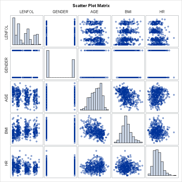
We see in the table above, that the typical subject in our dataset is more likely male, 70 years of age, with a bmi of 26.6 and heart rate of 87. The mean time to event (or loss to followup) is 882.4 days, not a particularly useful quantity. All of these variables vary quite a bit in these data. Most of the variables are at least slightly correlated with the other variables.
3. Nonparametric (Descriptive) Survival Analysis using proc lifetest
3.1. The Kaplan-Meier estimator of the survival function
3.1.1 Background: The Kaplan Meier Estimator:
The Kaplan_Meier survival function estimator is calculated as:
\[\hat S(t)=\prod_{t_i\leq t}\frac{n_i – d_i}{n_i}, \]
where \(n_i\) is the number of subjects at risk and \(d_i\) is the number of subjects who fail, both at time \(t_i\). Thus, each term in the product is the conditional probability of survival beyond time \(t_i\), meaning the probability of surviving beyond time \(t_i\), given the subject has survived up to time \(t_i\). The survival function estimate of the the unconditional probability of survival beyond time \(t\) (the probability of survival beyond time \(t\) from the onset of risk) is then obtained by multiplying together these conditional probabilities up to time \(t\) together.
Looking at the table of “Product-Limit Survival Estimates” below, for the first interval, from 1 day to just before 2 days, \(n_i\) = 500, \(d_i\) = 8, so \(\hat S(1) = \frac{500 – 8}{500} = 0.984\). The probability of surviving the next interval, from 2 days to just before 3 days during which another 8 people died, given that the subject has survived 2 days (the conditional probability) is \(\frac{492-8}{492} = 0.98374\). The unconditional probability of surviving beyond 2 days (from the onset of risk) then is \(\hat S(2) = \frac{500 – 8}{500}\times\frac{492-8}{492} = 0.984\times0.98374=.9680\)
3.1.2. Obtaining and interpreting tables of Kaplan-Meier Estimates from proc lifetest
Survival analysis often begins with examination of the overall survival experience through non-parametric methods, such as Kaplan-Meier (product-limit) and life-table estimators of the survival function. Non-parametric methods are appealing because no assumption of the shape of the survivor function nor of the hazard function need be made. However, nonparametric methods do not model the hazard rate directly nor do they estimate the magnitude of the effects of covariates.
In the code below, we show how to obtain a table and graph of the Kaplan-Meier estimator of the survival function from proc lifetest:
- At a minimum
proc lifetestrequires specification of a failure time variable, herelenfol, on thetimestatement. - Without further specification, SAS will assume all times reported are uncensored, true failures. Thus, because many observations in WHAS500 are right-censored, we also need to specify a censoring variable and the numeric code that identifies a censored observation, which is accomplished below with
"fstat(0)". All numbers within the parentheses are treated as indicators for censoring, which implies that all numbers excluded from the parentheses are treated as indicators that the event occurred. - We also specify the option
atriskon theproc lifeteststatement to display the number at risk in our sample at various time points.
proc lifetest data=whas500 atrisk outs=outwhas500;
time lenfol*fstat(0);
run;| Product-Limit Survival Estimates | ||||||||
|---|---|---|---|---|---|---|---|---|
| LENFOL | Number at Risk | Observed Events | Survival | Failure | Survival Standard Error | Number Failed | Number Left | |
| 0.00 | 500 | 0 | 1.0000 | 0 | 0 | 0 | 500 | |
| 1.00 | . | . | . | . | . | 1 | 499 | |
| 1.00 | . | . | . | . | . | 2 | 498 | |
| 1.00 | . | . | . | . | . | 3 | 497 | |
| 1.00 | . | . | . | . | . | 4 | 496 | |
| 1.00 | . | . | . | . | . | 5 | 495 | |
| 1.00 | . | . | . | . | . | 6 | 494 | |
| 1.00 | . | . | . | . | . | 7 | 493 | |
| 1.00 | 500 | 8 | 0.9840 | 0.0160 | 0.00561 | 8 | 492 | |
| 2.00 | . | . | . | . | . | 9 | 491 | |
| 2.00 | . | . | . | . | . | 10 | 490 | |
| 2.00 | . | . | . | . | . | 11 | 489 | |
| 2.00 | . | . | . | . | . | 12 | 488 | |
| 2.00 | . | . | . | . | . | 13 | 487 | |
| 2.00 | . | . | . | . | . | 14 | 486 | |
| 2.00 | . | . | . | . | . | 15 | 485 | |
| 2.00 | 492 | 8 | 0.9680 | 0.0320 | 0.00787 | 16 | 484 | |
| 3.00 | . | . | . | . | . | 17 | 483 | |
| 3.00 | . | . | . | . | . | 18 | 482 | |
| 3.00 | 484 | 3 | 0.9620 | 0.0380 | 0.00855 | 19 | 481 | |
Above we see the table of Kaplan-Meier estimates of the survival function produced by proc lifetest. Each row of the table corresponds to an interval of time, beginning at the time in the “LENFOL” column for that row, and ending just before the time in the “LENFOL” column in the first subsequent row that has a different “LENFOL” value. For example, the time interval represented by the first row is from 0 days to just before 1 day. In this interval, we can see that we had 500 people at risk and that no one died, as “Observed Events” equals 0 and the estimate of the “Survival” function is 1.0000. During the next interval, spanning from 1 day to just before 2 days, 8 people died, indicated by 8 rows of “LENFOL”=1.00 and by “Observed Events”=8 in the last row where “LENFOL”=1.00. It is important to note that the survival probabilities listed in the Survival column are unconditional, and are to be interpreted as the probability of surviving from the beginning of follow up time up to the number days in the LENFOL column.
Let’s take a look at later survival times in the table:
359.00 …..136364
| Product-Limit Survival Estimates | ||||||||
|---|---|---|---|---|---|---|---|---|
| LENFOL | Number at Risk | Observed Events | Survival | Failure | Survival Standard Error | Number Failed | Number Left | |
| 359.00 | 365 | 2 | 0.7260 | 0.2740 | 0.0199 | 137 | 363 | |
| 363.00 | 363 | 1 | 0.7240 | 0.2760 | 0.0200 | 138 | 362 | |
| 368.00 | * | 362 | 0 | . | . | . | 138 | 361 |
| 371.00 | * | . | 0 | . | . | . | 138 | 360 |
| 371.00 | * | . | 0 | . | . | . | 138 | 359 |
| 371.00 | * | 361 | 0 | . | . | . | 138 | 358 |
| 373.00 | * | 358 | 0 | . | . | . | 138 | 357 |
| 376.00 | * | . | 0 | . | . | . | 138 | 356 |
| 376.00 | * | 357 | 0 | . | . | . | 138 | 355 |
| 382.00 | 355 | 1 | 0.7220 | 0.2780 | 0.0200 | 139 | 354 | |
| 385.00 | 354 | 1 | 0.7199 | 0.2801 | 0.0201 | 140 | 353 | |
From “LENFOL”=368 to 376, we see that there are several records where it appears no events occurred. These are indeed censored observations, further indicated by the “*” appearing in the unlabeled second column. Subjects that are censored after a given time point contribute to the survival function until they drop out of the study, but are not counted as a failure. We can see this reflected in the survival function estimate for “LENFOL”=382. During the interval [382,385) 1 out of 355 subjects at-risk died, yielding a conditional probability of survival (the probability of survival in the given interval, given that the subject has survived up to the begininng of the interval) in this interval of \(\frac{355-1}{355}=0.9972\). We see that the uncoditional probability of surviving beyond 382 days is .7220, since \(\hat S(382)=0.7220=p(surviving~ up~ to~ 382~ days)\times0.9971831\), we can solve for \(p(surviving~ up~ to~ 382~ days)=\frac{0.7220}{0.9972}=.7240\). In the table above, we see that the probability surviving beyond 363 days = 0.7240, the same probability as what we calculated for surviving up to 382 days, which implies that the censored observations do not change the survival estimates when they leave the study, only the number at risk.
3.1.3. Graphing the Kaplan-Meier estimate
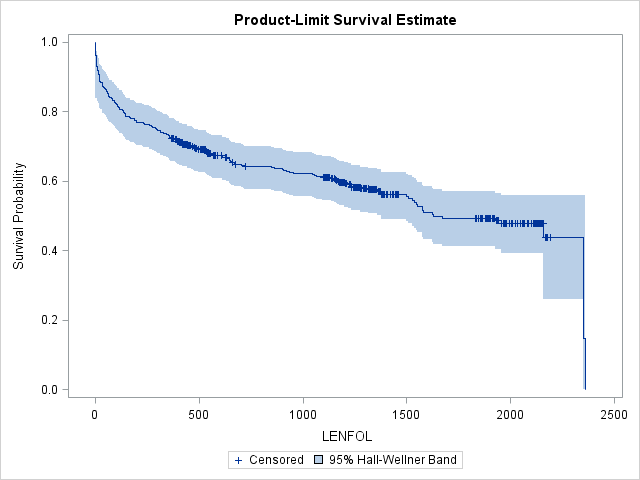
Graphs of the Kaplan-Meier estimate of the survival function allow us to see how the survival function changes over time and are fortunately very easy to generate in SAS:
- By default,
proc lifetestgraphs the Kaplan Meier estimate, even without theplot=option on theproc lifeteststatement, so we could have used the same code from above that produced the table of Kaplan-Meier estimates to generate the graph. - However, we would like to add confidence bands and the number at risk to the graph, so we add
plots=survival(atrisk cb).
proc lifetest data=whas500 atrisk plots=survival(cb) outs=outwhas500;
time lenfol*fstat(0);
run;
The step function form of the survival function is apparent in the graph of the Kaplan-Meier estimate. When a subject dies at a particular time point, the step function drops, whereas in between failure times the graph remains flat. The survival function drops most steeply at the beginning of study, suggesting that the hazard rate is highest immediately after hospitalization during the first 200 days. Censored observations are represented by vertical ticks on the graph. Notice the survival probability does not change when we encounter a censored observation. Because the observation with the longest follow-up is censored, the survival function will not reach 0. Instead, the survival function will remain at the survival probability estimated at the previous interval. The survival function is undefined past this final interval at 2358 days. The blue-shaded area around the survival curve represents the 95% confidence band, here Hall-Wellner confidence bands. This confidence band is calculated for the entire survival function, and at any given interval must be wider than the pointwise confidence interval (the confidence interval around a single interval) to ensure that 95% of all pointwise confidence intervals are contained within this band. Many transformations of the survivor function are available for alternate ways of calculating confidence intervals through the conftype option, though most transformations should yield very similar confidence intervals.
3.2. Nelson-Aalen estimator of the cumulative hazard function
Because of its simple relationship with the survival function, \(S(t)=e^{-H(t)}\), the cumulative hazard function can be used to estimate the survival function. The Nelson-Aalen estimator is a non-parametric estimator of the cumulative hazard function and is given by:
\[\hat H(t) = \sum_{t_i leq t}\frac{d_i}{n_i},\]
where \(d_i\) is the number who failed out of \(n_i\) at risk in interval \(t_i\). The estimator is calculated, then, by summing the proportion of those at risk who failed in each interval up to time \(t\).
- The Nelson-Aalen estimator is requested in SAS through the
nelsonoption on theproc lifeteststatement. SAS will output both Kaplan Meier estimates of the survival function and Nelson-Aalen estimates of the cumulative hazard function in one table.
proc lifetest data=whas500 atrisk nelson;
time lenfol*fstat(0);
run;| Survival Function and Cumulative Hazard Rate | ||||||||||
|---|---|---|---|---|---|---|---|---|---|---|
| LENFOL | Number at Risk | Observed Events | Product-Limit | Nelson-Aalen | Number Failed | Number Left | ||||
| Survival | Failure | Survival Standard Error | Cumulative Hazard | Cum Haz Standard Error | ||||||
| 0.00 | 500 | 0 | 1.0000 | 0 | 0 | 0 | . | 0 | 500 | |
| 1.00 | . | . | . | . | . | . | . | 1 | 499 | |
| 1.00 | . | . | . | . | . | . | . | 2 | 498 | |
| 1.00 | . | . | . | . | . | . | . | 3 | 497 | |
| 1.00 | . | . | . | . | . | . | . | 4 | 496 | |
| 1.00 | . | . | . | . | . | . | . | 5 | 495 | |
| 1.00 | . | . | . | . | . | . | . | 6 | 494 | |
| 1.00 | . | . | . | . | . | . | . | 7 | 493 | |
| 1.00 | 500 | 8 | 0.9840 | 0.0160 | 0.00561 | 0.0160 | 0.00566 | 8 | 492 | |
| 2.00 | . | . | . | . | . | . | . | 9 | 491 | |
| 2.00 | . | . | . | . | . | . | . | 10 | 490 | |
| 2.00 | . | . | . | . | . | . | . | 11 | 489 | |
| 2.00 | . | . | . | . | . | . | . | 12 | 488 | |
| 2.00 | . | . | . | . | . | . | . | 13 | 487 | |
| 2.00 | . | . | . | . | . | . | . | 14 | 486 | |
| 2.00 | . | . | . | . | . | . | . | 15 | 485 | |
| 2.00 | 492 | 8 | 0.9680 | 0.0320 | 0.00787 | 0.0323 | 0.00807 | 16 | 484 | |
| 3.00 | . | . | . | . | . | . | . | 17 | 483 | |
| 3.00 | . | . | . | . | . | . | . | 18 | 482 | |
| 3.00 | 484 | 3 | 0.9620 | 0.0380 | 0.00855 | 0.0385 | 0.00882 | 19 | 481 | |
Let’s confirm our understanding of the calculation of the Nelson-Aalen estimator by calculating the estimated cumulative hazard at day 3: \(\hat H(3)=\frac{8}{500} + \frac{8}{492} + \frac{3}{484} = 0.0385\), which matches the value in the table. The interpretation of this estimate is that we expect 0.0385 failures (per person) by the end of 3 days. The estimate of survival beyond 3 days based off this Nelson-Aalen estimate of the cumulative hazard would then be \(\hat S(3) = exp(-0.0385) = 0.9623\). This matches closely with the Kaplan Meier product-limit estimate of survival beyond 3 days of 0.9620. One can request that SAS estimate the survival function by exponentiating the negative of the Nelson-Aalen estimator, also known as the Breslow estimator, rather than by the Kaplan-Meier estimator through the method=breslow option on the proc lifetest statement. In very large samples the Kaplan-Meier estimator and the transformed Nelson-Aalen (Breslow) estimator will converge.
3.3. Calculating median, mean, and other survival times of interest in proc lifetest
Researchers are often interested in estimates of survival time at which 50% or 25% of the population have died or failed. Because of the positive skew often seen with followup-times, medians are often a better indicator of an “average” survival time. We obtain estimates of these quartiles as well as estimates of the mean survival time by default from proc lifetest. We see that beyond beyond 1,671 days, 50% of the population is expected to have failed. Notice that the interval during which the first 25% of the population is expected to fail, [0,297) is much shorter than the interval during which the second 25% of the population is expected to fail, [297,1671). This reinforces our suspicion that the hazard of failure is greater during the beginning of follow-up time.
proc lifetest data=whas500 atrisk nelson;
time lenfol*fstat(0);
run;| Quartile Estimates | ||||
|---|---|---|---|---|
| Percent | Point Estimate | 95% Confidence Interval | ||
| Transform | [Lower | Upper) | ||
| 75 | 2353.00 | LOGLOG | 2350.00 | 2358.00 |
| 50 | 1627.00 | LOGLOG | 1506.00 | 2353.00 |
| 25 | 296.00 | LOGLOG | 146.00 | 406.00 |
| Mean | Standard Error |
|---|---|
| 1417.21 | 48.14 |
3.4. Comparing survival functions using nonparametric tests
Suppose that you suspect that the survival function is not the same among some of the groups in your study (some groups tend to fail more quickly than others). One can also use non-parametric methods to test for equality of the survival function among groups in the following manner:
- When provided with a grouping variable in a
stratastatement inproc lifetest, SAS will produce graphs of the survival function (unless other graphs are requested) stratified by the grouping variable as well as tests of equality of the survival function across strata. For example, we could enter the class (categorical) variablegenderon thestratastatement to request that SAS compare the survival experiences of males and females.

proc lifetest data=whas500 atrisk plots=survival(atrisk cb) outs=outwhas500;
strata gender;
time lenfol*fstat(0);
run;| Test of Equality over Strata | |||
|---|---|---|---|
| Test | Chi-Square | DF | Pr > Chi-Square |
| Log-Rank | 7.7911 | 1 | 0.0053 |
| Wilcoxon | 5.5370 | 1 | 0.0186 |
| -2Log(LR) | 10.5120 | 1 | 0.0012 |
In the graph of the Kaplan-Meier estimator stratified by gender below, it appears that females generally have a worse survival experience. This is reinforced by the three significant tests of equality.
3.4.1. Background: Tests of equality of the survival function
In the output we find three Chi-square based tests of the equality of the survival function over strata, which support our suspicion that survival differs between genders. The calculation of the statistic for the nonparametric “Log-Rank” and “Wilcoxon” tests is given by :
\[Q = \frac{\bigg[\sum\limits_{i=1}^m w_j(d_{ij}-\hat e_{ij})\bigg]^2}{\sum\limits_{i=1}^m w_j^2\hat v_{ij}},\]
where \(d_{ij}\) is the observed number of failures in stratum \(i\) at time \(t_j\), \(\hat e_{ij}\) is the expected number of failures in stratum \(i\) at time \(t_j\), \(\hat v_{ij}\) is the estimator of the variance of \(d_{ij}\), and \(w_i\) is the weight of the difference at time \(t_j\) (see Hosmer and Lemeshow(2008) for formulas for \(\hat e_{ij}\) and \(\hat v_{ij}\)). In a nutshell, these statistics sum the weighted differences between the observed number of failures and the expected number of failures for each stratum at each timepoint, assuming the same survival function of each stratum. In other words, if all strata have the same survival function, then we expect the same proportion to die in each interval. If these proportions systematically differ among strata across time, then the \(Q\) statistic will be large and the null hypothesis of no difference among strata is more likely to be rejected.
The log-rank and Wilcoxon tests in the output table differ in the weights \(w_j\) used. The log-rank or Mantel-Haenzel test uses \(w_j = 1\), so differences at all time intervals are weighted equally. The Wilcoxon test uses \(w_j = n_j\), so that differences are weighted by the number at risk at time \(t_j\), thus giving more weight to differences that occur earlier in followup time. Other nonparametric tests using other weighting schemes are available through the test= option on the strata statement. The “-2Log(LR)” likelihood ratio test is a parametric test assuming exponentially distributed survival times and will not be further discussed in this nonparametric section.
3.5. Nonparametric estimation of the hazard function
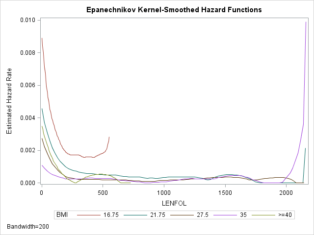
Standard nonparametric techniques do not typically estimate the hazard function directly. However, we can still get an idea of the hazard rate using a graph of the kernel-smoothed estimate. As the hazard function \(h(t)\) is the derivative of the cumulative hazard function \(H(t)\), we can roughly estimate the rate of change in \(H(t)\) by taking successive differences in \(\hat H(t)\) between adjacent time points, \(\Delta \hat H(t) = \hat H(t_j) – \hat H(t_{j-1})\). SAS computes differences in the Nelson-Aalen estimate of \(H(t)\). We generally expect the hazard rate to change smoothly (if it changes) over time, rather than jump around haphazardly. To accomplish this smoothing, the hazard function estimate at any time interval is a weighted average of differences within a window of time that includes many differences, known as the bandwidth. Widening the bandwidth smooths the function by averaging more differences together. However, widening will also mask changes in the hazard function as local changes in the hazard function are drowned out by the larger number of values that are being averaged together. Below is an example of obtaining a kernel-smoothed estimate of the hazard function across BMI strata with a bandwidth of 200 days:
- We request plots of the hazard function with a bandwidth of 200 days with
plot=hazard(bw=200) - SAS conveniently allows the creation of strata from a continuous variable, such as bmi, on the fly with the
stratastatement We specify the left endpoints of each bmi to form 5 bmi categories: 15-18.5, 18.5-25, 25-30, 30-40, and >40.
proc lifetest data=whas500 atrisk plots=hazard(bw=200) outs=outwhas500;
strata bmi(15,18.5,25,30,40);
time lenfol*fstat(0);
run;
The lines in the graph are labeled by the midpoint bmi in each group. From the plot we can see that the hazard function indeed appears higher at the beginning of follow-up time and then decreases until it levels off at around 500 days and stays low and mostly constant. The hazard function is also generally higher for the two lowest BMI categories. The sudden upticks at the end of follow-up time are not to be trusted, as they are likely due to the few number of subjects at risk at the end. The red curve representing the lowest BMI category is truncated on the right because the last person in that group died long before the end of followup time.
4. Background: The Cox proportional hazards regression model
4.1. Background: Estimating the hazard function, \(h(t)\)
Whereas with non-parametric methods we are typically studying the survival function, with regression methods we examine the hazard function, \(h(t)\). The hazard function for a particular time interval gives the probability that the subject will fail in that interval, given that the subject has not failed up to that point in time. The hazard rate can also be interpreted as the rate at which failures occur at that point in time, or the rate at which risk is accumulated, an interpretation that coincides with the fact that the hazard rate is the derivative of the cumulative hazard function, \(H(t)\).
In regression models for survival analysis, we attempt to estimate parameters which describe the relationship between our predictors and the hazard rate. We would like to allow parameters, the \(\beta\)s, to take on any value, while still preserving the non-negative nature of the hazard rate. A common way to address both issues is to parameterize the hazard function as:
\[h(t|x)=exp(\beta_0 + \beta_1x)\].
In this parameterization, \(h(t|x)\) is constrained to be strictly positive, as the exponential function always evaluates to positive, while \(\beta_0\) and \(\beta_1\) are allowed to take on any value. Notice, however, that \(t\) does not appear in the formula for the hazard function, thus implying that in this parameterization, we do not model the hazard rate’s dependence on time. A complete description of the hazard rate’s relationship with time would require that the functional form of this relationship be parameterized somehow (for example, one could assume that the hazard rate has an exponential relationship with time). However, in many settings, we are much less interested in modeling the hazard rate’s relationship with time and are more interested in its dependence on other variables, such as experimental treatment or age. For such studies, a semi-parametric model, in which we estimate regression parameters as covariate effects but ignore (leave unspecified) the dependence on time, is appropriate.
4.2. Background: The Cox proportional hazards model
We can remove the dependence of the hazard rate on time by expressing the hazard rate as a product of \(h_0(t)\), a baseline hazard rate which describes the hazard rates dependence on time alone, and \(r(x,\beta_x)\), which describes the hazard rates dependence on the other \(x\) covariates:
\[h(t)=h_0(t)r(x,\beta_x)\].
In this parameterization, \(h(t)\) will equal \(h_0(t)\) when \(r(x,\beta_x) = 1\). It is intuitively appealing to let \(r(x,\beta_x) = 1\) when all \(x = 0\), thus making the baseline hazard rate, \(h_0(t)\), equivalent to a regression intercept. Above, we discussed that expressing the hazard rate’s dependence on its covariates as an exponential function conveniently allows the regression coefficients to take on any value while still constraining the hazard rate to be positive. The exponential function is also equal to 1 when its argument is equal to 0. We will thus let \(r(x,\beta_x) = exp(x\beta_x)\), and the hazard function will be given by:
\[h(t)=h_0(t)exp(x\beta_x)\].
This parameterization forms the Cox proportional hazards model. It is called the proportional hazards model because the ratio of hazard rates between two groups with fixed covariates will stay constant over time in this model. For example, the hazard rate when time \(t\) when \(x = x_1\) would then be \(h(t|x_1) = h_0(t)exp(x_1\beta_x)\), and at time \(t\) when \(x = x_2\) would be \(h(t|x_2) = h_0(t)exp(x_2\beta_x)\). The covariate effect of \(x\), then is the ratio between these two hazard rates, or a hazard ratio(HR):
\[HR = \frac{h(t|x_2)}{h(t|x_1)} = \frac{h_0(t)exp(x_2\beta_x)}{h_0(t)exp(x_1\beta_x)}\]
Notice that the baseline hazard rate, \(h_0(t)\) is cancelled out, and that the hazard rate does not depend on time \(t\):
\[HR = exp(\beta_x(x_2-x_1))\]
The hazard rate \(HR\) will thus stay constant over time with fixed covariates. Because of this parameterization, covariate effects are multiplicative rather than additive and are expressed as hazard ratios, rather than hazard differences. As we see above, one of the great advantages of the Cox model is that estimating predictor effects does not depend on making assumptions about the form of the baseline hazard function, \(h_0(t)\), which can be left unspecified. Instead, we need only assume that whatever the baseline hazard function is, covariate effects multiplicatively shift the hazard function and these multiplicative shifts are constant over time.
Cox models are typically fitted by maximum likelihood methods, which estimate the regression parameters that maximize the probability of observing the given set of survival times. So what is the probability of observing subject \(i\) fail at time \(t_j\)? At the beginning of a given time interval \(t_j\), say there are \(R_j\) subjects still at-risk, each with their own hazard rates:
\[h(t_j|x_i)=h_0(t_j)exp(x_i\beta)\]
The probability of observing subject \(j\) fail out of all \(R_j\) remaing at-risk subjects, then, is the proportion of the sum total of hazard rates of all \(R_j\) subjects that is made up by subject \(j\)’s hazard rate. For example, if there were three subjects still at risk at time \(t_j\), the probability of observing subject 2 fail at time \(t_j\) would be:
\[Pr(subject=2|failure=t_j)=\frac{h(t_j|x_2)}{h(t_j|x_1)+h(t_j|x_2)+h(t_j|x_3)}\]
All of those hazard rates are based on the same baseline hazard rate \(h_0(t_i)\), so we can simplify the above expression to:
\[Pr(subject=2|failure=t_j)=\frac{exp(x_2\beta)}{exp(x_1\beta)+exp(x_2\beta)+exp(x_3\beta)}\]
We can similarly calculate the joint probability of observing each of the \(n\) subject’s failure times, or the likelihood of the failure times, as a function of the regression parameters, \(\beta\), given the subject’s covariates values \(x_j\):
\[L(\beta) = \prod_{j=1}^{n} \Bigg\lbrace\frac{exp(x_j\beta)}{\sum_{iin R_j}exp(x_i\beta)}\Bigg\rbrace\]
where \(R_j\) is the set of subjects still at risk at time \(t_j\). Maximum likelihood methods attempt to find the \(\beta\) values that maximize this likelihood, that is, the regression parameters that yield the maximum joint probability of observing the set of failure times with the associated set of covariate values. Because this likelihood ignores any assumptions made about the baseline hazard function, it is actually a partial likelihood, not a full likelihood, but the resulting \(\beta\) have the same distributional properties as those derived from the full likelihood.
.
5. Cox proportional hazards regression in SAS using proc phreg
5.1. Fitting a simple Cox regression model
We request Cox regression through proc phreg in SAS. Previously, we graphed the survival functions of males in females in the WHAS500 dataset and suspected that the survival experience after heart attack may be different between the two genders. Perhaps you also suspect that the hazard rate changes with age as well. Below we demonstrate a simple model in proc phreg, where we determine the effects of a categorical predictor, gender, and a continuous predictor, age on the hazard rate:
- To specify that
genderis a categorical predictor, we enter it on theclassstatement. - We also would like survival curves based on our model, so we add
plots=survivalto theproc phregstatement, although as we shall see this specification is probably insufficient for what we want. - On the
modelstatement, on the left side of the equation, we provide the follow up time variable, lenfol, and the censoring variable, fstat, with all censoring values listed in parentheses. On the right side of the equation we list all the predictors.
proc phreg data = whas500;
class gender;
model lenfol*fstat(0) = gender age;;
run;| Model Fit Statistics | ||
|---|---|---|
| Criterion | Without Covariates | With Covariates |
| -2 LOG L | 2455.158 | 2313.140 |
| AIC | 2455.158 | 2317.140 |
| SBC | 2455.158 | 2323.882 |
| Testing Global Null Hypothesis: BETA=0 | |||
|---|---|---|---|
| Test | Chi-Square | DF | Pr > ChiSq |
| Likelihood Ratio | 142.0177 | 2 | <.0001 |
| Score | 126.6381 | 2 | <.0001 |
| Wald | 119.3806 | 2 | <.0001 |
| Type 3 Tests | |||
|---|---|---|---|
| Effect | DF | Wald Chi-Square | Pr > ChiSq |
| GENDER | 1 | 0.2175 | 0.6410 |
| AGE | 1 | 116.3986 | <.0001 |
| Analysis of Maximum Likelihood Estimates | ||||||||
|---|---|---|---|---|---|---|---|---|
| Parameter | DF | Parameter Estimate | Standard Error | Chi-Square | Pr > ChiSq | Hazard Ratio | Label | |
| GENDER | Female | 1 | -0.06556 | 0.14057 | 0.2175 | 0.6410 | 0.937 | GENDER Female |
| AGE | 1 | 0.06683 | 0.00619 | 116.3986 | <.0001 | 1.069 | ||
The above output is only a portion of what SAS produces each time you run proc phreg. In particular we would like to highlight the following tables:
Model Fit Statistics: Displays fit statistics which are typically used for model comparison and selection. This is our first model, so we have no other model to compare with, except that by default SAS will display model fit statistics of a model with no predictors. We see here that adding gender and particularly age (as we will see below) as predictors improves the fit of the model, as all three statistics decreaseTesting Global Null Hypothesis: \(\BETA=0: Displays test of hypothesis that all coefficients in the model are 0, that is, an overall test of whether the model as a whole can predict changes in the hazard rate. These tests are asymptotically equivalent, but may differ in smaller samples, in which case the likelihood ratio test is generally preferred. Here the tests agree, and it appears that at least one of our regression coefficients is significantly different from 0.Analysis of Maximum Likelihood Estimates: Displays model coefficients, tests of significance, and exponentiated coefficient as hazard ratio. Here it appears that although females have a ~6% (Hazard Ratio = 0.937) decrease in the hazard rate compared to males, this decrease is not significant. On the other hand, with each year of age the hazard rate increases by 7% (Hazard Ratio = 1.069), a significant change. Our initial supsicion that the hazard rates were different between genders seems to be wrong once we account for age effects (females are generally older in this dataset), but as shall see the effects are more nuanced. Also notice that there is no intercept. In Cox regression, the intercept is absorbed into the baseline hazard function, which is left unspecified.
5.2. Producing graphs of the survival and baseline hazard function after Cox regression
Handily, proc phreg has pretty extensive graphing capabilities.< Below is the graph and its accompanying table produced by simply adding plots=survival to the proc phreg statement.
- When only
plots=survivalis specified on theproc phregstatement, SAS will produce one graph, a “reference curve” of the survival function at the reference level of all categorical predictors and at the mean of all continuous predictors.
proc phreg data=whas500 plots=survival;
class gender;
model lenfol*fstat(0) = gender age;;
run;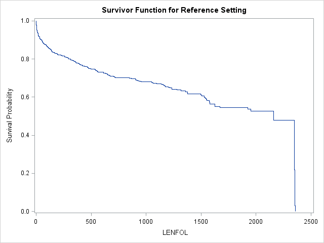
| Reference Set of Covariates for Plotting | |
|---|---|
| AGE | GENDER |
| 69.845947 | Male |
In this model, this reference curve is for males at age 69.845947 Usually, we are interested in comparing survival functions between groups, so we will need to provide SAS with some additional instructions to get these graphs.
5.2.1. Use the baseline statement to generate survival plots by group
Acquiring more than one curve, whether survival or hazard, after Cox regression in SAS requires use of the baseline statement in conjunction with the creation of a small dataset of covariate values at which to estimate our curves of interest. Here are the typical set of steps to obtain survival plots by group:
- First, a dataset of covariate values is created in a
datastep. Each row contains a set of covariate values for which we would like a survival plot. - This dataset name is then specified on the
covariates=option on thebaselinestatement. Internally, SAS will expand the dataset to contain one observation at each event time per set of covariate values in thecovariates=dataset. - This expanded dataset can be named and then viewed with the
out=option, but obtaining theout=dataset is not at all necessary to generate the survival plots. - Two options on the
baselinestatement control grouping in the graphs. If a variable is specified aftergroup=(not used until later in the seminar), SAS will create separate graphs for each level of that variable. If a variable is specified after therowid=option, SAS will create separate lines within the same plot for each level of this variable. Thegroup=androwid=options on thebaselinestatment work in tandem with the(overlay=group)option specified immediately after theplotsoption on theproc phregstatement. Ifplots(overlay=group)is specified, and there is a variable specified on thegroup=option on thebaselinestatement, SAS will create separate graphs by level of that variable. If additionally a variable is specified on therowid=option on thebaselinestatement, SAS will plot separate lines by this variable in each plot. If nogroup=option is used, we can still get separate lines by therowid=variable on one plot by specifying no type of overlaying like so:plots(overlay)=. Omitting the(overlay)completely will tell SAS to create separate graphs byrowid=. - Both survival and cumulative hazard curves are available using the
plots=option on theproc phregstatement, with the keywordssurvivalandcumhaz, respectively.
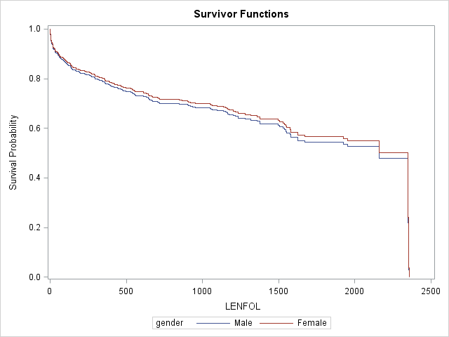
Let’s get survival curves (cumulative hazard curves are also available) for males and female at the mean age of 69.845947 in the manner we just described.
- We use a
datastep to create a dataset called “covs” with 2 rows of covariates - We then specify “covs” on
covariates=option on thebaselinestatement. There are 326 discrete event times in the WHAS500 dataset, so thebaselinestatement will then expand thecovariates=dataset so that we have 326 entries each for males and females at the mean age. - We specify the name of the output dataset, “base”, that contains our covariate values at each event time on the
out=option - We request survival plots that are overlaid with the
plot(overlay)=(survival)specification on theproc phregstatement. If we did not specify(overlay), SAS would produce separate graphs for males and females. - We also add the
rowid=option on thebaselinestatement, which tells SAS to label the curves on our graph using the variablegender.
proc format;
value gender 0 = "male" 1 = "female";
run;
data covs;
format gender gender.;
input gender age;
datalines;
0 69.845947
1 69.845947
;
run;

proc phreg data = whas500 plots(overlay)=(survival);
class gender;
model lenfol*fstat(0) = gender age;
baseline covariates=covs out=base / rowid=gender;
run;
;
The survival curves for females is slightly higher than the curve for males, suggesting that the survival experience is possibly slightly better (if significant) for females, after controlling for age. The estimated hazard ratio of .937 comparing females to males is not significant.
5.3. Expanding and interpreting the Cox regression model with interaction terms
In our previous model we examined the effects of gender and age on the hazard rate of dying after being hospitalized for heart attack. At this stage we might be interested in expanding the model with more predictor effects. For example, we found that the gender effect seems to disappear after accounting for age, but we may suspect that the effect of age is different for each gender. We could test for different age effects with an interaction term between gender and age. Based on past research, we also hypothesize that BMI is predictive of the hazard rate, and that its effect may be non-linear. Finally, we strongly suspect that heart rate is predictive of survival, so we include this effect in the model as well.
In the code below we fit a Cox regression model where we allow examine the effects of gender, age, bmi, and heart rate on the hazard rate. Here, we would like to introdue two types of interaction:
- The interaction of 2 different variables, such as gender and age, is specified through the syntax
gender|age, which requests inidividual effects of each term as well as their interaction. This allows the effect of age to differ by gender (and the effect of gender to differ by age). - The interaction of a continuous variable, such as bmi, with itself is specified by
bmi|bmi, to model both linear and quadratic effects of that variable. A quadratic effect implies that the effect of the variable changes with the level of the variable itself (i.e. an interaction of the variable with itself).
proc phreg data = whas500;
format gender gender.;
class gender;
model lenfol*fstat(0) = gender|age bmi|bmi hr ;
run;| Model Fit Statistics | ||
|---|---|---|
| Criterion | Without Covariates | With Covariates |
| -2 LOG L | 2455.158 | 2276.150 |
| AIC | 2455.158 | 2288.150 |
| SBC | 2455.158 | 2308.374 |
| Testing Global Null Hypothesis: BETA=0 | |||
|---|---|---|---|
| Test | Chi-Square | DF | Pr > ChiSq |
| Likelihood Ratio | 179.0077 | 6 | <.0001 |
| Score | 174.7924 | 6 | <.0001 |
| Wald | 154.9497 | 6 | <.0001 |
| Type 3 Tests | |||
|---|---|---|---|
| Effect | DF | Wald Chi-Square | Pr > ChiSq |
| GENDER | 1 | 4.5117 | 0.0337 |
| AGE | 1 | 72.0368 | <.0001 |
| AGE*GENDER | 1 | 5.4646 | 0.0194 |
| BMI | 1 | 7.0382 | 0.0080 |
| BMI*BMI | 1 | 4.8858 | 0.0271 |
| HR | 1 | 21.4528 | <.0001 |
| Analysis of Maximum Likelihood Estimates | ||||||||
|---|---|---|---|---|---|---|---|---|
| Parameter | DF | Parameter Estimate | Standard Error | Chi-Square | Pr > ChiSq | Hazard Ratio | Label | |
| GENDER | Female | 1 | 2.10986 | 0.99330 | 4.5117 | 0.0337 | . | GENDER Female |
| AGE | 1 | 0.07086 | 0.00835 | 72.0368 | <.0001 | . | ||
| AGE*GENDER | Female | 1 | -0.02925 | 0.01251 | 5.4646 | 0.0194 | . | GENDER Female * AGE |
| BMI | 1 | -0.23323 | 0.08791 | 7.0382 | 0.0080 | . | ||
| BMI*BMI | 1 | 0.00363 | 0.00164 | 4.8858 | 0.0271 | . | BMI * BMI | |
| HR | 1 | 0.01277 | 0.00276 | 21.4528 | <.0001 | 1.013 | ||
We would probably prefer this model to the simpler model with just gender and age as explanatory factors for a couple of reasons. First, each of the effects, including both interactions, are significant. Second, all three fit statistics, -2 LOG L, AIC and SBC, are each 20-30 points lower in the larger model, suggesting the including the extra parameters improve the fit of the model substantially.
Let’s interpret our model. We should begin by analyzing our interactions. The significant AGE*GENDER interaction term suggests that the effect of age is different by gender. Recall that when we introduce interactions into our model, each individual term comprising that interaction (such as GENDER and AGE) is no longer a main effect, but is instead the simple effect of that variable with the interacting variable held at 0. Thus, for example the AGE term describes the effect of age when gender=0, or the age effect for males. It appears that for males the log hazard rate increases with each year of age by 0.07086, and this AGE effect is significant, AGE*GENDER term is negative, which means for females, the change in the log hazard rate per year of age is 0.07086-0.02925=0.04161. We cannot tell whether this age effect for females is significantly different from 0 just yet (see below), but we do know that it is significantly different from the age effect for males. Similarly, because we included a BMI*BMI interaction term in our model, the BMI term is interpreted as the effect of bmi when bmi is 0. The BMI*BMI term describes the change in this effect for each unit increase in bmi. Thus, it appears, that when bmi=0, as bmi increases, the hazard rate decreases, but that this negative slope flattens and becomes more positive as bmi increases.
5.4. Using the hazardratio statement and graphs to interpret effects, particularly interactions
Notice in the Analysis of Maximum Likelihood Estimates table above that the Hazard Ratio entries for terms involved in interactions are left empty. SAS omits them to remind you that the hazard ratios corresponding to these effects depend on other variables in the model.
Below, we show how to use the hazardratio statement to request that SAS estimate 3 hazard ratios at specific levels of our covariates.
- After the keyword
hazardratio, we can optionally apply a label, then we specify the variable whose levels are to be compared in the hazard, and finally after the option keywordatwe tell SAS at which level of our other covariates to evaluate this hazard ratio. If the variable whose hazard rates are to computed is not involved in an interaction, specification of additional covariates is unncessary since the hazard ratio is constant across levels of all other covariates (a main effect). - We calculate the hazard ratio describing a one-unit increase in age, or \(\frac{HR(age+1)}{HR(age)}\), for both genders. Notice the
=ALLfollowinggender, which is used only withclassvariables to request the hazard ratio at all levels of the class variable. - We also calculate the hazard ratio between females and males, or \(\frac{HR(gender=1)}{HR(gender=0)}\) at ages 0, 20, 40, 60, and 80.
- Finally, we calculate the hazard ratio describing a 5-unit increase in bmi, or \(\frac{HR(bmi+5)}{HR(bmi)}\), at clinically revelant BMI scores. Notice the additional option
units=5.BMIclasses are typically separated by about 5 points, so we would like to see how the hazard ratio between (approximately) adjacent BMI classes changes asbmiincreases.
proc phreg data = whas500;
class gender;
model lenfol*fstat(0) = gender|age bmi|bmi hr ;
hazardratio 'Effect of 1-unit change in age by gender' age / at(gender=ALL);
hazardratio 'Effect of gender across ages' gender / at(age=(0 20 40 60 80));
hazardratio 'Effect of 5-unit change in bmi across bmi' bmi / at(bmi = (15 18.5 25 30 40)) units=5;
run;
| Effect of 1-unit change in age by gender: Hazard Ratios for AGE | |||
|---|---|---|---|
| Description | Point Estimate | 95% Wald Confidence Limits | |
| AGE Unit=1 At GENDER=Female | 1.042 | 1.022 | 1.063 |
| AGE Unit=1 At GENDER=Male | 1.073 | 1.056 | 1.091 |
| Effect of gender across ages: Hazard Ratios for GENDER | |||
|---|---|---|---|
| Description | Point Estimate | 95% Wald Confidence Limits | |
| GENDER Female vs Male At AGE=0 | 8.247 | 1.177 | 57.783 |
| GENDER Female vs Male At AGE=20 | 4.594 | 1.064 | 19.841 |
| GENDER Female vs Male At AGE=40 | 2.559 | 0.955 | 6.857 |
| GENDER Female vs Male At AGE=60 | 1.426 | 0.837 | 2.429 |
| GENDER Female vs Male At AGE=80 | 0.794 | 0.601 | 1.049 |
| Effect of 5-unit change in bmi across bmi: Hazard Ratios for BMI | |||
|---|---|---|---|
| Description | Point Estimate | 95% Wald Confidence Limits | |
| BMI Unit=5 At BMI=15 | 0.588 | 0.428 | 0.809 |
| BMI Unit=5 At BMI=18.5 | 0.668 | 0.535 | 0.835 |
| BMI Unit=5 At BMI=25 | 0.846 | 0.733 | 0.977 |
| BMI Unit=5 At BMI=30 | 1.015 | 0.797 | 1.291 |
| BMI Unit=5 At BMI=40 | 1.459 | 0.853 | 2.497 |
In each of the tables, we have the hazard ratio listed under Point Estimate and confidence intervals for the hazard ratio. Confidence intervals that do not include the value 1 imply that hazard ratio is significantly different from 1 (and that the log hazard rate change is significanlty different from 0). Thus, in the first table, we see that the hazard ratio for age, \(\frac{HR(age+1)}{HR(age)}\), is lower for females than for males, but both are significantly different from 1. Thus, both genders accumulate the risk for death with age, but females accumulate risk more slowly. In the second table, we see that the hazard ratio between genders, \(\frac{HR(gender=1)}{HR(gender=0)}\), decreases with age, significantly different from 1 at age = 0 and age = 20, but becoming non-signicant by 40. We previously saw that the gender effect was modest, and it appears that for ages 40 and up, which are the ages of patients in our dataset, the hazard rates do not differ by gender. Finally, we see that the hazard ratio describing a 5-unit increase in bmi, \(\frac{HR(bmi+5)}{HR(bmi)}\), increases with bmi. The effect of bmi is significantly lower than 1 at low bmi scores, indicating that higher bmi patients survive better when patients are very underweight, but that this advantage disappears and almost seems to reverse at higher bmi levels.
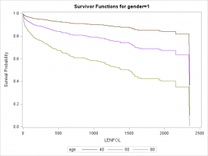
Graphs are particularly useful for interpreting interactions. We can plot separate graphs for each combination of values of the covariates comprising the interactions. Below we plot survivor curves across several ages for each gender through the follwing steps:
- We again first create a
covariatesdataset, here calledcovs2, to tell SAS at which covariate values we would like to estimate the survivor function. Here we want curves for both males and females at ages 40, 60, and 80. All predictors in the model must be in thecovariatesdataset, so we setbmiandhrto their means. - We then specify the name of this dataset in the
covariates=option on thebaselinestatement. - We request separate lines for each age using
rowid=and separate graphs by gender usinggroup=on thebaselinestatement. - We request that SAS create separate survival curves by the
groupoption, with separate curves byrowid=overlaid on the same graph with the syntaxplots(overlay=group)=(survival).
data covs2;
format gender gender.;
input gender age bmi hr;
datalines;
0 40 26.614 87.018
0 60 26.614 87.018
0 80 26.614 87.018
1 40 26.614 87.018
1 60 26.614 87.018
1 80 26.614 87.018
;
run;

proc phreg data = whas500 plots(overlay=group)=(survival);
class gender;
model lenfol*fstat(0) = gender|age bmi|bmi hr ;
baseline covariates=covs2  / rowid=age group=gender;
run;
As we surmised earlier, the effect of age appears to be more severe in males than in females, reflected by the greater separation between curves in the top graph.
5.5. Create time-varying covariates with programming statements
Thus far in this seminar we have only dealt with covariates with values fixed across follow up time. With such data, each subject can be represented by one row of data, as each covariate only requires only value. However, often we are interested in modeling the effects of a covariate whose values may change during the course of follow up time. For example, patients in the WHAS500 dataset are in the hospital at the beginnig of follow-up time, which is defined by hospital admission after heart attack. Many, but not all, patients leave the hospital before dying, and the length of stay in the hospital is recorded in the variable los. We, as researchers, might be interested in exploring the effects of being hospitalized on the hazard rate. As we know, each subject in the WHAS500 dataset is represented by one row of data, so the dataset is not ready for modeling time-varying covariates. Our goal is to transform the data from its original state:
| Obs | ID | LENFOL | FSTAT | LOS |
|---|---|---|---|---|
| 1 | 1 | 2178 | 0 | 5 |
| 2 | 2 | 2172 | 0 | 5 |
| 3 | 3 | 2190 | 0 | 5 |
| 4 | 4 | 297 | 1 | 10 |
| 5 | 5 | 2131 | 0 | 6 |
| 6 | 6 | 1 | 1 | 1 |
| 7 | 7 | 2122 | 0 | 5 |
to an expanded state that can accommodate time-varying covariates, like this (notice the new variable in_hosp):
| Obs | ID | start | stop | status | in_hosp |
|---|---|---|---|---|---|
| 1 | 1 | 0 | 5 | 0 | 1 |
| 2 | 1 | 5 | 2178 | 0 | 0 |
| 3 | 2 | 0 | 5 | 0 | 1 |
| 4 | 2 | 5 | 2172 | 0 | 0 |
| 5 | 3 | 0 | 5 | 0 | 1 |
| 6 | 3 | 5 | 2190 | 0 | 0 |
| 7 | 4 | 0 | 10 | 0 | 1 |
| 8 | 4 | 10 | 297 | 1 | 0 |
| 9 | 5 | 0 | 6 | 0 | 1 |
| 10 | 5 | 6 | 2131 | 0 | 0 |
| 11 | 6 | 0 | 1 | 1 | 1 |
| 12 | 7 | 0 | 5 | 0 | 1 |
| 13 | 7 | 5 | 2122 | 0 | 0 |
Notice the creation of start and stop variables, which denote the beginning and end intervals defined by hospitalization and death (or censoring). Notice also that care must be used in altering the censoring variable to accommodate the multiple rows per subject. To specify a Cox model with start and stop times for each interval, due to the usage of time-varying covariates, we need to specify the start and stop time in the model statement:
proc phreg data = whas500;
model (start, stop)*status(0) = in_hosp ;
run;
If the data come prepared with one row of data per subject each time a covariate changes value, then the researcher does not need to expand the data any further. However, if that is not the case, then it may be possible to use programming statement within proc phreg to create variables that reflect the changing the status of a covariate. Alternatively, the data can be expanded in a data step, but this can be tedious and prone to errors (although instructive, on the other hand).
Fortunately, it is very simple to create a time-varying covariate using programming statements in proc phreg. These statement essentially look like data step statements, and function in the same way. In the code below, we model the effects of hospitalization on the hazard rate. To do so:
- We create the variable
in_hosp, which is 1 if the patient is currently in the hospital (lenfol<=los), and 0 when the patient leaves (lenfol>los). - We also add the newly created time-varying covariate to the
modelstatement.
proc phreg data = whas500;
format gender gender.;
class gender;
model lenfol*fstat(0) = gender|age bmi|bmi hr in_hosp ;
if lenfol > los then in_hosp = 0;
else in_hosp = 1;
run;
| Analysis of Maximum Likelihood Estimates | ||||||||
|---|---|---|---|---|---|---|---|---|
| Parameter | DF | Parameter Estimate | Standard Error | Chi-Square | Pr > ChiSq | Hazard Ratio | Label | |
| GENDER | Female | 1 | 2.16143 | 1.00426 | 4.6322 | 0.0314 | . | GENDER Female |
| AGE | 1 | 0.07301 | 0.00851 | 73.6642 | <.0001 | . | ||
| AGE*GENDER | Female | 1 | -0.03025 | 0.01266 | 5.7090 | 0.0169 | . | GENDER Female * AGE |
| BMI | 1 | -0.22302 | 0.08847 | 6.3548 | 0.0117 | . | ||
| BMI*BMI | 1 | 0.00348 | 0.00166 | 4.4123 | 0.0357 | . | BMI * BMI | |
| HR | 1 | 0.01222 | 0.00277 | 19.4528 | <.0001 | 1.012 | ||
| in_hosp | 1 | 2.09971 | 0.39617 | 28.0906 | <.0001 | 8.164 | ||
It appears that being in the hospital increases the hazard rate, but this is probably due to the fact that all patients were in the hospital immediately after heart attack, when they presumbly are most vulnerable.
6. Exploring functional form of covariates
In the Cox proportional hazards model, additive changes in the covariates are assumed to have constant multiplicative effects on the hazard rate (expressed as the hazard ratio (\(HR\))):
\[HR = exp(\beta_x(x_2-x_1))\]
In other words, each unit change in the covariate, no matter at what level of the covariate, is associated with the same percent change in the hazard rate, or a constant hazard ratio. For example, if \(\beta_x\) is 0.5, each unit increase in \(x\) will cause a ~65% increase in the hazard rate, whether X is increasing from 0 to 1 or from 99 to 100, as \(HR = exp(0.5(1)) = 1.6487\). However, it is quite possible that the hazard rate and the covariates do not have such a loglinear relationship. Constant multiplicative changes in the hazard rate may instead be associated with constant multiplicative, rather than additive, changes in the covariate, and might follow this relationship:
\[HR = exp(\beta_x(log(x_2)-log(x_1)) = exp(\beta_x(log\frac{x_2}{x_1}))\]
This relationship would imply that moving from 1 to 2 on the covariate would cause the same percent change in the hazard rate as moving from 50 to 100.
It is not always possible to know a priori the correct functional form that describes the relationship between a covariate and the hazard rate. Plots of the covariate versus martingale residuals can help us get an idea of what the functional from might be.
6.1 Plotting cumulative martingale residuals against covariates to determine the functional form of covariates
The background necessary to explain the mathematical definition of a martingale residual is beyond the scope of this seminar, but interested readers may consult (Therneau, 1990). For this seminar, it is enough to know that the martingale residual can be interpreted as a measure of excess observed events, or the difference between the observed number of events and the expected number of events under the model:
\[martingale~ residual = excess~ observed~ events = observed~ events – (expected~ events|model)\]
Therneau and colleagues(1990) show that the smooth of a scatter plot of the martingale residuals from a null model (no covariates at all) versus each covariate individually will often approximate the correct functional form of a covariate. Previously we suspected that the effect of bmi on the log hazard rate may not be purely linear, so it would be wise to investigate further. In the code below we demonstrate the steps to take to explore the functional form of a covariate:
- Run a null Cox regression model by leaving the right side of equation empty on the
modelstatement withinproc phreg. - Save the martingale residuals to an output dataset using the
resmartoption in theoutputstatement withinproc phreg. In the code below we save the residuals to a variable named “martingale”. - Use
proc loessto plot scatter plot smooths of the covariate (here bmi) vs the martingale residuals. The loess method selects portions of the data into local neighborhoods and fits a regression surface to each neighboorhood. This allows the regression surface to take a wide variety of shapes. The smoothed regression surfaces should approximate the functional form of the covariate. - Within
proc loesswe specify the martingale residual dataset on theproc loessstatement. We specify which variables to model on themodelstatement. - The fraction of the data contained in each neighborhood is determined by the smoothing parameter, and thus larger smoothing parameter values produce smoother surfaces. Below we request 4 smooths using the
smoothoption. - A desirable feature of loess smooth is that the residuals from the regression do not have any structure. We can examine residual plots for each smooth (with loess smooth themselves) by specifying the
plots=ResidualsBySmoothoption on theproc loessstatement.
proc phreg data = whas500;
class gender;
model lenfol*fstat(0) = ;
output out=residuals resmart=martingale;
run;

proc loess data = residuals plots=ResidualsBySmooth(smooth);
model martingale = bmi / smooth=0.2 0.4 0.6 0.8;
run;
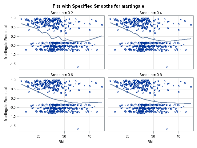
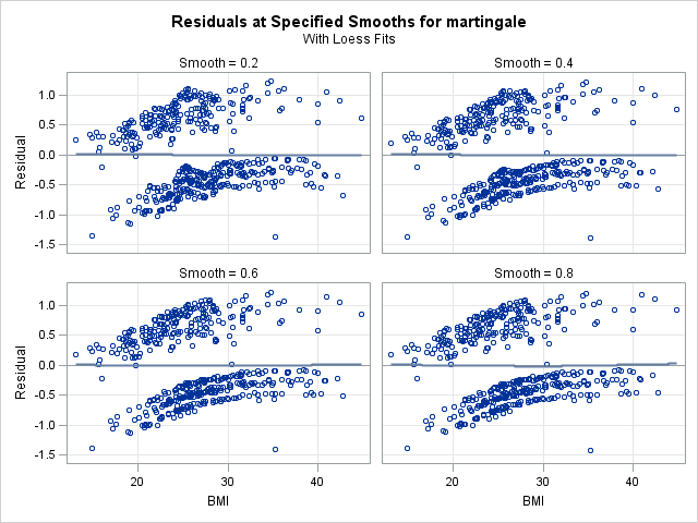
In the left panel above, “Fits with Specified Smooths for martingale”, we see our 4 scatter plot smooths. In all of the plots, the martingale residuals tend to be larger and more positive at low bmi values, and smaller and more negative at high bmi values. This indicates that omitting bmi from the model causes those with low bmi values to modeled with too low a hazard rate (as the number of observed events is in excess of the expected number of events). On the right panel, “Residuals at Specified Smooths for martingale”, are the smoothed residual plots, all of which appear to have no structure. The surface where the smoothing parameter=0.2 appears to be overfit and jagged, and such a shape would be difficult to model. However, each of the other 3 at the higher smoothing parameter values have very similar shapes, which appears to be a linear effect of bmi that flattens as bmi increases. This indicates that our choice of modeling a linear and quadratic effect of bmi was a reasonable one. One caveat is that this method for determining functional form is less reliable when covariates are correlated. However, despite our knowledge that bmi is correlated with age, this method provides good insight into bmi’s functional form.
6.2. Using the assess statement to explore functional forms
SAS provides built-in methods for evaluating the functional form of covariates through its assess statement. These techniques were developed by Lin, Wei and Zing (1993). The basic idea is that martingale residuals can be grouped cumulatively either by follow up time and/or by covariate value. If our Cox model is correctly specified, these cumulative martingale sums should randomly fluctuate around 0. Significant departures from random error would suggest model misspecification. We could thus evaluate model specification by comparing the observed distribution of cumulative sums of martingale residuals to the expected distribution of the residuals under the null hypothesis that the model is correctly specified. The null distribution of the cumulative martingale residuals can be simulated through zero-mean Gaussian processes. If the observed pattern differs significantly from the simulated patterns, we reject the null hypothesis that the model is correctly specified, and conclude that the model should be modified. In such cases, the correct form may be inferred from the plot of the observed pattern. This technique can detect many departures from the true model, such as incorrect functional forms of covariates (discussed in this section), violations of the proportional hazards assumption (discussed later), and using the wrong link function (not discussed).
Below we demonstrate use of the assess statement to the functional form of the covariates. Several covariates can be evaluated simultaneously. We compare 2 models, one with just a linear effect of bmi and one with both a linear and quadratic effect of bmi (in addition to our other covariates). Using the assess statement to check functional form is very simple:
- List all covariates whose functional forms are to be checked within parentheses after
var=on theassessstatement. Only continuous covariates may be assessed this way, not class variables. - We also specify the
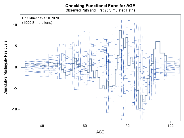
resampleoption, which performs a supremum test of the null hypothesis that the observed pattern of martingale residuals is not different from the expected pattern (i.e. that the model is correctly specified). Essentially, the supremum tests calculates the proportion of 1000 simulations that contain a maximum cumulative martingale residual larger than the observed maximum cumulative residual. This proportion is reported as the p-value. If only a small proportion, say 0.05, of the simulations have a maximum cumulative residual larger than the observed maximum, then that suggests that the observed residuals are larger than expected under the proposed model and that the model should be modified.
First let’s look at the model with just a linear effect for bmi.
proc phreg data = whas500;
class gender;
model lenfol*fstat(0) = gender|age bmi hr;
assess var=(age bmi hr) / resample;
run;
| Supremum Test for Functional Form | ||||
|---|---|---|---|---|
| Variable | Maximum Absolute Value | Replications | Seed | Pr > MaxAbsVal |
| AGE | 11.2240 | 1000 | 164727001 | 0.1510 |
| BMI | 11.0212 | 1000 | 164727001 | 0.2440 |
| HR | 9.3459 | 1000 | 164727001 | 0.3940 |
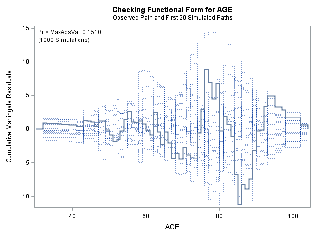
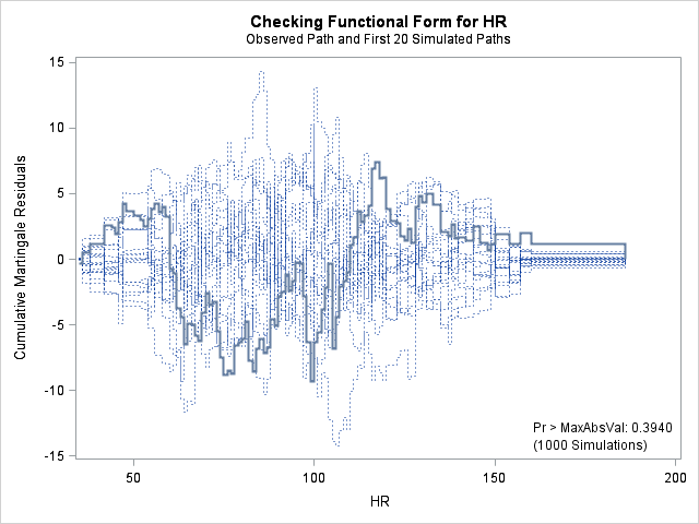
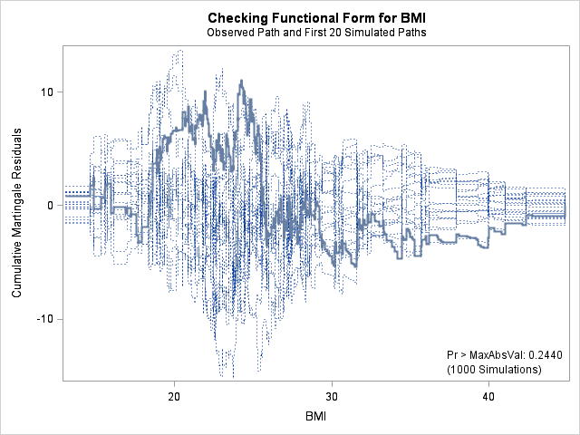
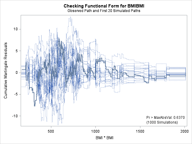
In each of the graphs above, a covariate is plotted against cumulative martingale residuals. The solid lines represent the observed cumulative residuals, while dotted lines represent 20 simulated sets of residuals expected under the null hypothesis that the model is correctly specified. Unless the seed option is specified, these sets will be different each time proc phreg is run. A solid line that falls significantly outside the boundaries set up collectively by the dotted lines suggest that our model residuals do not conform to the expected residuals under our model. None of the graphs look particularly alarming (click here to see an alarming graph in the SAS example on assess). Additionally, none of the supremum tests are significant, suggesting that our residuals are not larger than expected. Nevertheless, the bmi graph at the top right above does not look particularly random, as again we have large positive residuals at low bmi values and smaller negative residuals at higher bmi values. This suggests that perhaps the functional form of bmi should be modified.
Now let’s look at the model with just both linear and quadratic effects for bmi.
proc phreg data = whas500;
class gender;
model lenfol*fstat(0) = gender|age bmi|bmi hr;
assess var=(age bmi bmi*bmi hr) / resample;
run;
| Supremum Test for Functional Form | ||||
|---|---|---|---|---|
| Variable | Maximum Absolute Value | Replications | Seed | Pr > MaxAbsVal |
| AGE | 9.7412 | 1000 | 179001001 | 0.2820 |
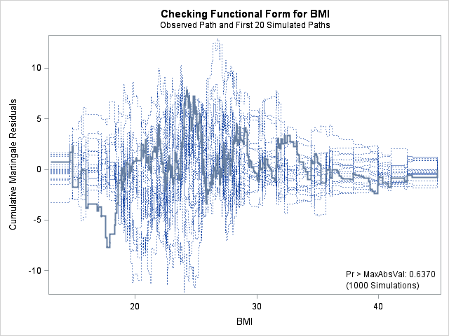
| BMI | 7.8329 | 1000 | 179001001 | 0.6370 |
| BMIBMI | 7.8329 | 1000 | 179001001 | 0.6370 |
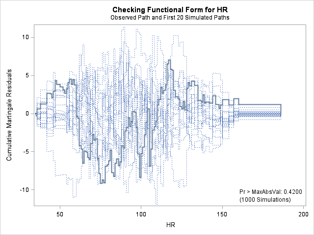
| HR | 9.1548 | 1000 | 179001001 | 0.4200 |
The graph for bmi at top right looks better behaved now with smaller residuals at the lower end of bmi. The other covariates, including the additional graph for the quadratic effect for bmi all look reasonable. Thus, we again feel justified in our choice of modeling a quadratic effect of bmi.
7. Assessing the proportional hazards assumption
A central assumption of Cox regression is that covariate effects on the hazard rate, namely hazard ratios, are constant over time. For example, if males have twice the hazard rate of females 1 day after followup, the Cox model assumes that males have twice the hazard rate at 1000 days after follow up as well. Violations of the proportional hazard assumption may cause bias in the estimated coefficients as well as incorrect inference regarding significance of effects.
7.1. Graphing Kaplan-Meier survival function estimates to assess proportional hazards for categorical covariates
In the case of categorical covariates, graphs of the Kaplan-Meier estimates of the survival function provide quick and easy checks of proportional hazards. If proportional hazards holds, the graphs of the survival function should look “parallel”, in the sense that they should have basically the same shape, should not cross, and should start close and then diverge slowly through follow up time. Earlier in the seminar we graphed the Kaplan-Meier survivor function estimates for males and females, and gender appears to adhere to the proportional hazards assumption.

proc lifetest data=whas500 atrisk plots=survival(atrisk cb) outs=outwhas500;
strata gender;
time lenfol*fstat(0);
run;
7.2. Plotting scaled Schoenfeld residuals vs functions of time to assess proportional hazards of a continuous covariate
A popular method for evaluating the proportional hazards assumption is to examine the Schoenfeld residuals. The Schoenfeld residual for observation \(j\) and covariate \(p\) is defined as the difference between covariate \(p\) for observation \(j\) and the weighted average of the covariate values for all subjects still at risk when observation \(j\) experiences the event. Grambsch and Therneau (1994) show that a scaled version of the Schoenfeld residual at time \(k\) for a particular covariate \(p\) will approximate the change in the regression coefficient at time \(k\):
\[E(s^\star_{kp}) + \hat{\beta}_p \approx \beta_j(t_k)\]
In the relation above, \(s^\star_{kp}\) is the scaled Schoenfeld residual for covariate \(p\) at time \(k\), \(\beta_p\) is the time-invariant coefficient, and \(\beta_j(t_k)\) is the time-variant coefficient. In other words, the average of the Schoenfeld residuals for coefficient \(p\) at time \(k\) estimates the change in the coefficient at time \(k\). Thus, if the average is 0 across time, then that suggests the coefficient \(p\) does not vary over time and that the proportional hazards assumption holds for covariate \(p\). It is possible that the relationship with time is not linear, so we should check other functional forms of time, such as log(time) and rank(time).
We will use scatterplot smooths to explore the scaled Schoenfeld residuals’ relationship with time, as we did to check functional forms before. Here are the steps we will take to evaluate the proportional hazards assumption for age through scaled Schoenfeld residuals:
- Scaled Schoenfeld residuals are obtained in the output dataset, so we will need to supply the name of an output dataset using the
out=option on theoutputstatement as before. Below, we call this dataset “schoen”. - SAS provides Schoenfeld residuals for each covariate, and they are output in the same order as the coefficients are listed in the “Analysis of Maximum Likelihood Estimates” table. Only as many residuals are output as names are supplied on the
ressch=option. For this demonstration, we are particularly interested in the Schoenfeld residuals for age. - We should check for non-linear relationships with time, so we include a
datastep that calculates the log oflenfol. Other functions can be explored as well. - We then use
proc loessto obtain our smooths. Flat lines at 0 suggest that the coefficient does not vary over time and that proportional hazards holds.
proc phreg data=whas500;
class gender;
model lenfol*fstat(0) = gender|age bmi|bmi hr;
output out=schoen ressch=schgender schage schgenderage
   schbmi schbmibmi schhr;
run;

data schoen;
set schoen;
loglenfol = log(lenfol);
run;

proc loess data = schoen;
model schage=lenfol / smooth=(0.2 0.4 0.6 0.8);
run;
proc loess data = schoen;
model schage=loglenfol / smooth=(0.2 0.4 0.6 0.8);
run;
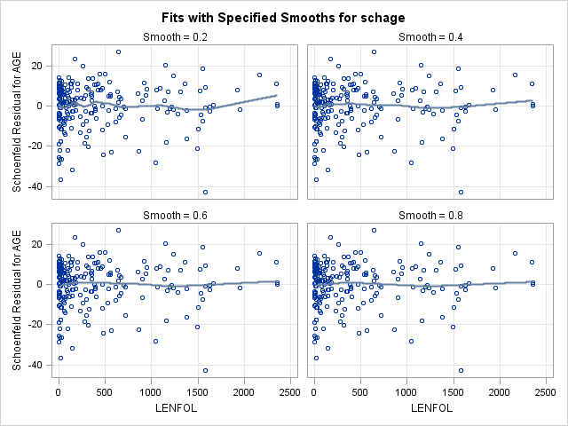
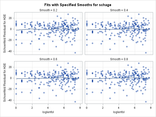
Although possibly slightly positively trending, the smooths appear mostly flat at 0, suggesting that the coefficient for age does not change over time and that proportional hazards holds for this covariate. The same procedure could be repeated to check all covariates.
7.3. Using assess with the ph option to check proportional hazards
The procedure Lin, Wei, and Zing(1990) developed that we previously introduced to explore covariate functional forms can also detect violations of proportional hazards by using a transform of the martingale residuals known as the empirical score process. Once again, the empirical score process under the null hypothesis of no model misspecification can be approximated by zero mean Gaussian processes, and the observed score process can be compared to the simulated processes to asses departure from proportional hazards.
The assess statement with the ph option provides an easy method to assess the proportional hazards assumption both graphically and numerically for many covariates at once. Here we demonstrate how to assess the proportional hazards assumption for all of our covariates (graph for gender not shown):
proc phreg data=whas500;
class gender;
model lenfol*fstat(0) = gender|age bmi|bmi hr;
assess var=(age bmi bmi*bmi hr) ph / resample ;
run;- As before with checking functional forms, we list all the variables for which we would like to assess the proportional hazards assumption after the
varoption on theassessstatement. - We additionally add the option
phto tell SAS that we would like to assess proportional hazards in addition to checking functional forms. - As before, we specify the
resampleoption to request the supremum tests of the null hypothesis that proportional hazards holds. These tests calculate the proportion of simulated score processes that yielded a maximum score larger than the maximum observed score process. A very small proportion (p-value) suggests violation of proportional hazards.
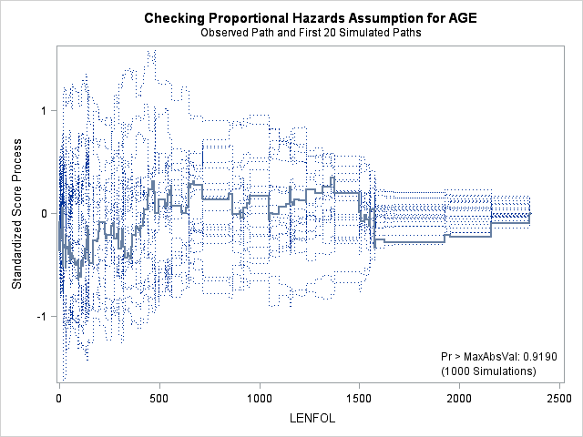
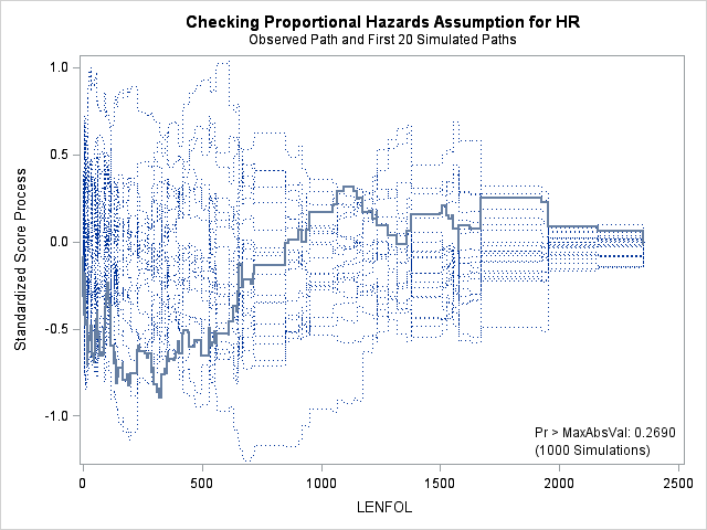
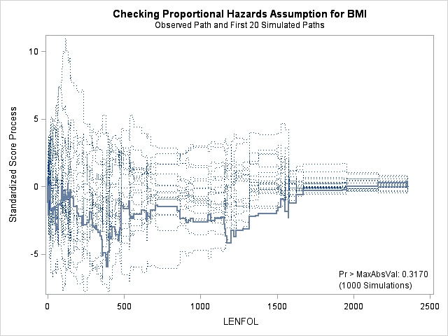
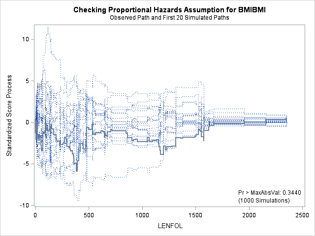
| Supremum Test for Proportionals Hazards Assumption | ||||
|---|---|---|---|---|
| Variable | Maximum Absolute Value | Replications | Seed | Pr > MaxAbsVal |
| GENDERFemale | 0.6394 | 1000 | 778428000 | 0.7680 |
| AGE | 0.4965 | 1000 | 778428000 | 0.9600 |
| BMI | 5.9813 | 1000 | 778428000 | 0.2890 |
| BMIBMI | 5.9350 | 1000 | 778428000 | 0.3160 |
| HR | 0.8861 | 1000 | 778428000 | 0.3080 |
As we did with functional form checking, we inspect each graph for observed score processes, the solid blue lines, that appear quite different from the 20 simulated score processes, the dotted lines. None of the solid blue lines looks particularly aberrant, and all of the supremum tests are non-significant, so we conclude that proportional hazards holds for all of our covariates.
7.4. Dealing with nonproportionality
If nonproportional hazards are detected, the researcher has many options with how to address the violation (Therneau & Grambsch, 2000):
- Ignore the nonproportionality if it appears the changes in the coefficient over time are very small or if it appears the outliers are driving the changes in the coefficient. In large datasets, very small departures from proportional hazards can be detected. If, say, a regression coefficient changes only by 1% over time, it is unlikely that any overarching conclusions of the study would be affected. Additionally, a few heavily influential points may be causing nonproportional hazards to be detected, so it is important to use graphical methods to ensure this is not the case.
- Stratify the model by the nonproportional covariate. Stratification allows each stratum to have its own baseline hazard, which solves the problem of nonproportionality. However, one cannot test whether the stratifying variable itself affects the hazard rate significantly. Additionally, although stratifying by a categorical covariate works naturally, it is often difficult to know how to best discretize a continuous covariate. This can be easily accomplished in
proc phrehwith thestratastatement. - Run Cox models on intervals of follow up time rather than on its entirety. Proportional hazards may hold for shorter intervals of time within the entirety of follow up time. Some data management will be required to ensure that everyone is properly censored in each interval.
- Include covariate interactions with time as predictors in the Cox model. This can be accomplished through programming statements in
proc phreg, as these interactions are time-varying covariates themselves. Indeed, including such an interaction has been used as a test of proportional hazards — a significant interaction indicates violation of the assumption. Below, we provide code that shows how to include a covariate interaction with time in the model. We create the interaction variablehrtimeby multiplyinghrbylenfol. The interaction variable is of course included on themodelstatement as well. The output indicates that this interaction is non-significant, which is not surprising given thathrhas not shown evidence of nonproportionality.
proc phreg data=whas500;
class gender;
model lenfol*fstat(0) = gender|age bmi|bmi hr hrtime;
hrtime = hr*lenfol;
run;
| Analysis of Maximum Likelihood Estimates | ||||||||
|---|---|---|---|---|---|---|---|---|
| Parameter | DF | Parameter Estimate | Standard Error | Chi-Square | Pr > ChiSq | Hazard Ratio | Label | |
| GENDER | Female | 1 | 2.10602 | 0.99264 | 4.5013 | 0.0339 | . | GENDER Female |
| AGE | 1 | 0.07099 | 0.00835 | 72.2933 | <.0001 | . | ||
| AGE*GENDER | Female | 1 | -0.02927 | 0.01250 | 5.4805 | 0.0192 | . | GENDER Female * AGE |
| BMI | 1 | -0.23297 | 0.08788 | 7.0276 | 0.0080 | . | ||
| BMI*BMI | 1 | 0.00363 | 0.00164 | 4.8856 | 0.0271 | . | BMI * BMI | |
| HR | 1 | 0.01174 | 0.00350 | 11.2671 | 0.0008 | 1.012 | ||
| hrtime | 1 | 2.84574E-6 | 5.88882E-6 | 0.2335 | 0.6289 | 1.000 | ||
8. Influence Diagnostics
8.1. Inspecting \(df\beta\) to assess influence of observations on individual regression coefficients
After fitting a model it is good practice to assess the influence of observations in your data, to check if any outlier has a disproportionately large impact on the model. Once outliers are identified, we then decide whether to keep the observation or throw it out, because perhaps the data may have been entered in error or the observation is not particularly representative of the population of interest.
The dfbeta measure, \(df\beta\), quantifies how much an observation influences the regression coefficients in the model. For observation \(j\), \(df\beta_j\) approximates the change in a coefficient when that observation is deleted. We thus calculate the coefficient with the observation, call it \(\beta\), and then the coefficient when observation \(j\) is deleted, call it \(\beta_j\), and take the difference to obtain \(df\beta_j\).
\[df\beta_j \approx \hat{\beta} – \hat{\beta_j}\]
Positive values of \(df\beta_j\) indicate that the exclusion of the observation causes the coefficient to decrease, which implies that inclusion of the observation causes the coefficient to increase. Thus, it might be easier to think of \(df\beta_j\) as the effect of including observation \(j\) on the the coefficient.
SAS provides easy ways to examine the \(df\beta\) values for all observations across all coefficients in the model. Plots of covariates vs dfbetas can help to identify influential outliers. Here are the steps we use to assess the influence of each observation on our regression coefficients:
- We obtain \(df\beta_j\) values through in output datasets in SAS, so we will need to specify an
outputstatement withinproc phreg. On theoutputstatement, we supply the name of the output dataset “dfbeta” on theout=option. - There are \(df\beta_j\) values associated with each coefficient in the model, and they are output to the output dataset in the order that they appear in the parameter table “Analysis of Maximum Likelihood Estimates” (see above). The order of \(df\beta_j\) in the current model are: gender, age, gender*age, bmi, bmi*bmi, hr. SAS expects individual names for each \(df\beta_j\)associated with a coefficient. If only \(k\) names are supplied and \(k\) is less than the number of distinct df\betas, SAS will only output the first \(k\) \(df\beta_j\). Thus, to pull out all 6 \(df\beta_j\), we must supply 6 variable names for these \(df\beta_j\).
- We then plot each\(df\beta_j\) against the associated coviarate using
proc sgplot. Our aim is identifying which observations are influential, so we replace the marker symbol with theidnumber of the observation by specifying the variableidon themarkerchar=option.
proc phreg data = whas500;
class gender;
model lenfol*fstat(0) = gender|age bmi|bmi hr;
output out = dfbeta dfbeta=dfgender dfage dfagegender dfbmi dfbmibmi dfhr;
run;

proc sgplot data = dfbeta;
scatter x = age y=dfage / markerchar=id;
run;
proc sgplot data = dfbeta;
scatter x = bmi y=dfbmi / markerchar=id;
run;
proc sgplot data = dfbeta;
scatter x = bmi y=dfbmibmi / markerchar=id;
run;
proc sgplot data = dfbeta;
scatter x = hr y=dfhr / markerchar=id;
run;
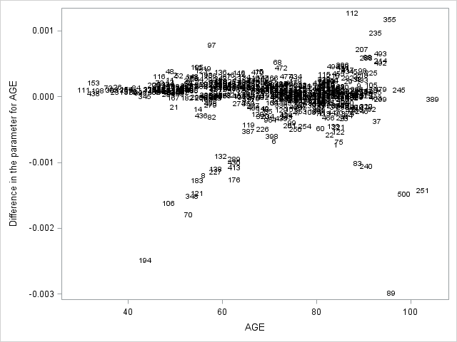
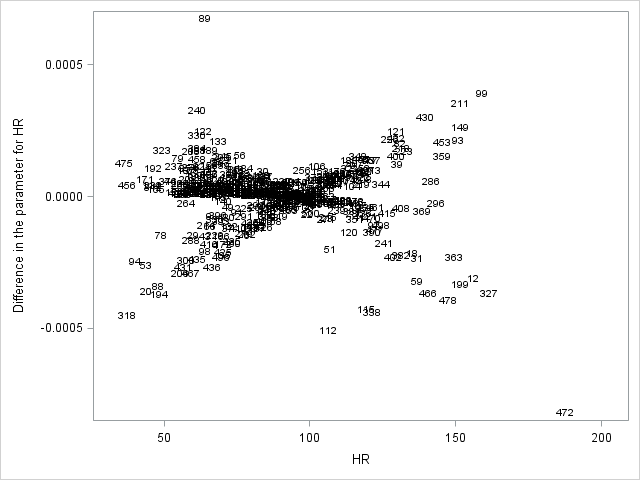
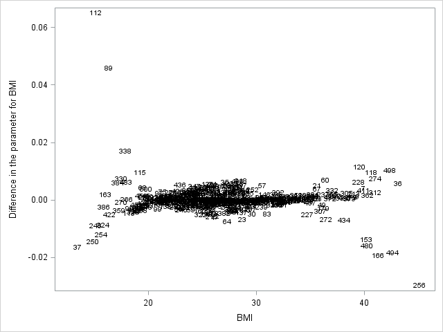
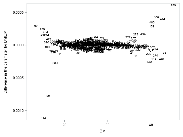
The dfbetas for age and hr look small compared to regression coefficients themselves (\(\hat{\beta}_{age}=0.07086\) and \(\hat{\beta}_{hr}=0.01277\)) for the most part, but id=89 has a rather large, negative dfbeta for hr. We also identify id=89 again and id=112 as influential on the linear bmi coefficient (\(\hat{\beta}_{bmi}=-0.23323\)), and their large positive dfbetas suggest they are pulling up the coefficient for bmi when they are included.
Once you have identified the outliers, it is good practice to check that their data were not incorrectly entered. These two observations, id=89 and id=112, have very low but not unreasonable bmi scores, 15.9 and 14.8. However they lived much longer than expected when considering their bmi scores and age (95 and 87), which attenuates the effects of very low bmi. Thus, we can expect the coefficient for bmi to be more severe or more negative if we exclude these observations from the model. Indeed, exclusion of these two outliers causes an almost doubling of \(\hat{\beta}_{bmi}\), from -0.23323 to -0.39619. Still, although their effects are strong, we believe the data for these outliers are not in error and the significance of all effects are unaffected if we exclude them, so we include them in the model.
proc print data = whas500(where=(id=112 or id=89));
var lenfol gender age bmi hr;
run;
| Obs | LENFOL | GENDER | AGE | BMI | HR |
|---|---|---|---|---|---|
| 89 | 1553 | Male | 95 | 15.9270 | 62 |
| 112 | 2123 | Female | 87 | 14.8428 | 105 |
proc phreg data = whas500(where=(id^=112 and id^=89));
class gender;
model lenfol*fstat(0) = gender|age bmi|bmi hr;
output out = dfbeta dfbeta=dfgender dfage dfagegender dfbmi dfbmibmi dfhr;
run;
| Analysis of Maximum Likelihood Estimates | ||||||||
|---|---|---|---|---|---|---|---|---|
| Parameter | DF | Parameter Estimate | Standard Error | Chi-Square | Pr > ChiSq | Hazard Ratio | Label | |
| GENDER | Female | 1 | 2.07605 | 1.01218 | 4.2069 | 0.0403 | . | GENDER Female |
| AGE | 1 | 0.07412 | 0.00855 | 75.2370 | <.0001 | . | ||
| AGE*GENDER | Female | 1 | -0.02959 | 0.01277 | 5.3732 | 0.0204 | . | GENDER Female * AGE |
| BMI | 1 | -0.39619 | 0.09365 | 17.8985 | <.0001 | . | ||
| BMI*BMI | 1 | 0.00640 | 0.00171 | 14.0282 | 0.0002 | . | BMI * BMI | |
| HR | 1 | 0.01244 | 0.00279 | 19.9566 | <.0001 | 1.013 | ||
8.2. Plotting likelihood displacement scores to assess influence on the overall model
Not only are we interested in how influential observations affect coefficients, we are interested in how they affect the model as a whole. The likelihood displacement score quantifies how much the likelihood of the model, which is affected by all coefficients, changes when the observation is left out. This analysis proceeds in much the same was as dfbeta analysis, in that we will:
- Output the likelihood displacement scores to an output dataset, which we name on the
out=option on theoutputstatement inproc phreg. Below, we name the output dataset “ld”. - Name the variable to store the likelihood displacement score on the
ld=option on theoutputstatement - Graph the likelihood displacement scores vs follow up time using
proc sgplot. We replace the marker symbols with the id number using themarkerchar=option again.
proc phreg data = whas500;
class gender;
model lenfol*fstat(0) = gender|age bmi|bmi hr;
output out=ld ld=ld;
run;

proc sgplot data=ld;
scatter x=lenfol y=ld / markerchar=id;
run;
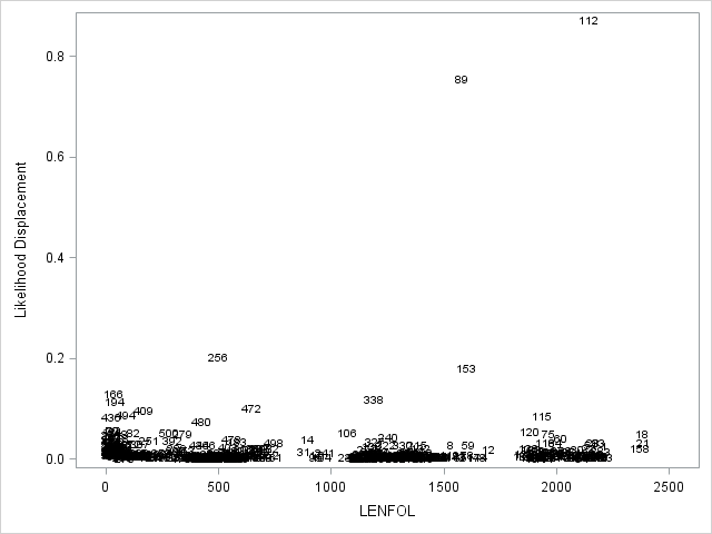
We see the same 2 outliers we identifed before, id=89 and id=112, as having the largest influence on the model overall, probably primarily through their effects on the bmi coefficient. However, we have decided that there covariate scores are reasonable so we retain them in the model.
References
Therneau, TM, Grambsch, PM. (2000). Modeling Survival Data: Extending the Cox Model. Springer: New York. Note: This was the primary reference used for this seminar. It contains numerous examples in SAS and R.
Grambsch, PM, Therneau, TM. (1994). Proportional hazards tests and diagnostics based on weighted residuals. Biometrika. 81. 515-526.
Grambsch, PM, Therneau, TM, Fleming TR. (1995). Diagnostic plots to reveal functional form for covariates in multiplicative intensity models. Biometrics. 51. 1469-82.
Hosmer, DW, Lemeshow, S, May S. (2008). Applied Survival Analysis. Wiley: Hoboken.
Lin, DY, Wei, LJ, Ying, Z. (1993). Checking the Cox model with cumulative sums of martingale-based residuals. Biometrika. 80(30). 557-72.
Therneau, TM, Grambsch PM, Fleming TR (1990). Martingale-based residuals for survival models. Biometrika. 77(1). 147-60.

