
Chapter Outline
1.0 Introduction
1.1 A First Regression Analysis
1.2 Examining Data
1.3 Simple linear regression
1.4 Multiple regression
1.5 Transforming variables
1.6 Summary
1.7 For more information
1.0 Introduction
This web book is composed of
four chapters covering a variety of topics about using SAS for regression. We should
emphasize that this book is about "data analysis" and that it demonstrates how
SAS can be used for regression analysis, as opposed to a book that covers the statistical
basis of multiple regression. We assume that you have had at least one statistics
course covering regression analysis and that you have a regression book that you can use
as a reference (see the Regression With SAS page and our Statistics Books for Loan page for recommended regression
analysis books). This book is designed to apply your knowledge of regression, combine it
with instruction on SAS, to perform, understand and interpret regression analyses.
This first chapter will cover topics in simple and multiple regression, as well as the
supporting tasks that are important in preparing to analyze your data, e.g., data
checking, getting familiar with your data file, and examining the distribution of your
variables. We will illustrate the basics of simple and multiple regression and
demonstrate the importance of inspecting, checking and verifying your data before accepting
the results of your analysis. In general, we hope to show that the results of your
regression analysis can be misleading without further probing of your data, which could
reveal relationships that a casual analysis could overlook.
In this chapter, and in subsequent chapters, we will be using a data file that was
created by randomly sampling 400 elementary schools from the California Department of
Education’s API 2000 dataset. This data file contains a measure of school academic
performance as well as other attributes of the elementary schools, such as, class size,
enrollment, poverty, etc.
You can access this data file over the web by clicking on elemapi.sas7bdat, or by visiting the
Regression
with SAS page where you can download all of the data files used in all of
the chapters of this book. The examples will assume you have stored your
files in a folder called c:sasreg,
but actually you can store the files in any folder you choose, but if you run
these examples be sure to change c:sasreg to
the name of the folder you have selected.
1.1 A First Regression Analysis
Let’s dive right in and perform a regression analysis using the variables api00,
acs_k3, meals and full. These measure the academic performance of the
school (api00), the average class size in kindergarten through 3rd grade (acs_k3),
the percentage of students receiving free meals (meals) – which is an indicator of
poverty, and the percentage of teachers who have full teaching credentials (full).
We expect that better academic performance would be associated with lower class size, fewer
students receiving free meals, and a higher percentage of teachers having full teaching
credentials. Below, we use proc reg for running
this regression model
followed by the SAS output.
proc reg data="c:sasregelemapi";
  model api00 = acs_k3 meals full;
run;

The REG Procedure
Model: MODEL1
Dependent Variable: api00 api 2000

                             Analysis of Variance

                                    Sum of           Mean
Source                   DF        Squares         Square    F Value    Pr > F

Model                     3        2634884         878295     213.41    <.0001
Error                   309        1271713     4115.57673
Corrected Total         312        3906597


Root MSE             64.15276    R-Square     0.6745
Dependent Mean      596.40575    Adj R-Sq     0.6713
Coeff Var            10.75656


                                    Parameter Estimates

                                            Parameter       Standard
Variable     Label                  DF       Estimate          Error    t Value    Pr > |t|

Intercept    Intercept               1      906.73916       28.26505      32.08      <.0001
acs_k3       avg class size k-3      1       -2.68151        1.39399      -1.92      0.0553
meals        pct free meals          1       -3.70242        0.15403     -24.04      <.0001
full         pct full credential     1        0.10861        0.09072       1.20      0.2321
Let’s focus on the three predictors, whether they are statistically significant and, if
so, the direction of the relationship. The average class size (acs_k3, b=-2.68), is
not significant (p=0.0553), but only just so, and the coefficient is negative which would
indicate that larger class sizes is related to lower academic performance — which is what
we would expect. Next, the effect of meals (b=-3.70, p<.0001) is significant
and its coefficient is negative indicating that the greater the proportion students
receiving free meals, the lower the academic performance. Please note, that we are
not saying that free meals are causing lower academic performance. The meals
variable is highly related to income level and functions more as a proxy for poverty.
Thus, higher levels of poverty are associated with lower academic performance. This result
also makes sense. Finally, the percentage of teachers with full credentials (full,
b=0.11, p=.2321) seems to be unrelated to academic performance. This would seem to indicate
that the percentage of teachers with full credentials is not an important factor in
predicting academic performance — this result was somewhat unexpected.
Should we take these results and write them up for publication? From these
results, we would conclude that lower class sizes are related to higher performance, that
fewer students receiving free meals is associated with higher performance, and that the
percentage of teachers with full credentials was not related to academic performance in
the schools. Before we write this up for publication, we should do a number of
checks to make sure we can firmly stand behind these results. We start by getting
more familiar with the data file, doing preliminary data checking, looking for errors in
the data.
1.2 Examining data
First, let’s use proc contents to learn more about this data file.
We can verify how many observations it has and see the names of the variables it contains.
proc contents data="c:sasregelemapi" ;
run;
The CONTENTS Procedure

Data Set Name: c:sasregelemapi                       Observations:         400
Member Type:   DATA                                    Variables:            21
Engine:        V8                                      Indexes:              0
Created:       4:58 Saturday, January 9, 1960          Observation Length:   83
Last Modified: 4:58 Saturday, January 9, 1960          Deleted Observations: 0
Protection:                                            Compressed:           NO
Data Set Type:                                         Sorted:               NO
Label:


     -----Engine/Host Dependent Information-----

Data Set Page Size:         8192
Number of Data Set Pages:   5
First Data Page:            1
Max Obs per Page:           98
Obs in First Data Page:     56
Number of Data Set Repairs: 0
File Name:                  c:sasregelemapi.sas7bdat
Release Created:            7.0000M0
Host Created:               WIN_NT


            -----Alphabetic List of Variables and Attributes-----

 #    Variable    Type    Len    Pos    Label
-----------------------------------------------------------------------------
11    acs_46      Num       3     39    avg class size 4-6
10    acs_k3      Num       3     36    avg class size k-3
 3    api00       Num       4     12    api 2000
 4    api99       Num       4     16    api 1999
17    avg_ed      Num       8     57    avg parent ed
15    col_grad    Num       3     51    parent college grad
 2    dnum        Num       4      8    district number
 7    ell         Num       3     27    english language learners
19    emer        Num       3     73    pct emer credential
20    enroll      Num       4     76    number of students
18    full        Num       8     65    pct full credential
16    grad_sch    Num       3     54    parent grad school
 5    growth      Num       4     20    growth 1999 to 2000
13    hsg         Num       3     45    parent hsg
21    mealcat     Num       3     80    Percentage free meals in 3 categories
 6    meals       Num       3     24    pct free meals
 9    mobility    Num       3     33    pct 1st year in school
12    not_hsg     Num       3     42    parent not hsg
 1    snum        Num       8      0    school number
14    some_col    Num       3     48    parent some college
 8    yr_rnd      Num       3     30    year round school
We will not go into all of the details of this output. Note that there are 400
observations and 21 variables. We have variables about academic performance in 2000
and 1999 and the change in performance, api00, api99 and growth
respectively. We also have various characteristics of the schools, e.g., class size,
parents education, percent of teachers with full and emergency credentials, and number of
students. Note that when we did our original regression analysis it said that there
were 313 observations, but the proc contents output indicates that we have 400
observations in the data file.
If you want to learn more about the data file, you could use proc print
to show some of the
observations. For example, below we proc print to show the first five observations.
proc print data="c:sasregelemapi"(obs=5) ;
run;
                              m             s c g
                               o        n    o o r                   m
                    g       y  b  a  a  o    m l a    a           e  e
            a   a   r  m    r  i  c  c  t    e _ d    v           n  a
     s   d  p   p   o  e    _  l  s  s  _    _ g _    g     f  e  r  l
 O   n   n  i   i   w  a  e r  i  _  _  h  h c r s    _     u  m  o  c
 b   u   u  0   9   t  l  l n  t  k  4  s  s o a c    e     l  e  l  a
 s   m   m  0   9   h  s  l d  y  3  6  g  g l d h    d     l  r  l  t

  1 906 41 693 600 93 67  9 0 11 16 22  0  0 0 0 0  .      76 24 247 2
  2 889 41 570 501 69 92 21 0 33 15 32  0  0 0 0 0  .      79 19 463 3
  3 887 41 546 472 74 97 29 0 36 17 25  0  0 0 0 0  .      68 29 395 3
  4 876 41 571 487 84 90 27 0 27 20 30 36 45 9 9 0 1.91000 87 11 418 3
  5 888 41 478 425 53 89 30 0 44 18 31 50 50 0 0 0 1.50000 87 13 520 3
This takes up lots of space on the page, but does not give us a lot of
information. Listing our data can be very helpful, but it is more helpful if you list
just the variables you are interested in. Let’s list the first 10
observations for the variables that we looked at in our first regression analysis.
proc print data="c:sasregelemapi"(obs=10) ;
  var api00 acs_k3 meals full;
run;
Obs    api00    acs_k3    meals    full
  1     693       16        67       76
  2     570       15        92       79
  3     546       17        97       68
  4     571       20        90       87
  5     478       18        89       87
  6     858       20         .      100
  7     918       19         .      100
  8     831       20         .       96
  9     860       20         .      100
 10     737       21        29       96
We see that among the first 10 observations, we have four missing values for meals.
It is likely that the missing data for meals had something to do with the
fact that the number of observations in our first regression analysis was 313 and not 400.
Another useful tool for learning about your variables is proc means.
Below we use proc means to learn more about the variables api00, acs_k3,
meals, and full.
proc means data="c:sasregelemapi";
  var api00 acs_k3 meals full;
run;
The MEANS Procedure

Variable  Label                  N          Mean       Std Dev       Minimum
----------------------------------------------------------------------------
api00     api 2000             400   647.6225000   142.2489610   369.0000000
acs_k3    avg class size k-3   398    18.5477387     5.0049328   -21.0000000
meals     pct free meals       315    71.9936508    24.3855697     6.0000000
full      pct full credential  400    66.0568000    40.2979258     0.4200000
----------------------------------------------------------------------------

Variable  Label                     Maximum
-------------------------------------------
api00     api 2000              940.0000000
acs_k3    avg class size k-3     25.0000000
meals     pct free meals        100.0000000
full      pct full credential   100.0000000
-------------------------------------------
We see that the api00 scores don’t have any missing values (because
the N is 400) and the scores range from 369-940. This makes sense since
the api scores can range from 200 to 1000. We see that the average class
size (acs_k3) had 398 valid values ranging from -21 to 25 and 2 are
missing. It seems odd for a class size to be -21. The percent receiving free
meals (meals) ranges from 6 to 100, but there are only 315 valid values
(85 are missing). This seems like a large number of missing values. The
percent with full credentials (full) ranges from .42 to 100 with no
missing.
We can also use proc freq to learn more about any categorical
variables, such as yr_rnd, as shown below.
proc freq data="c:sasregelemapi";
  tables yr_rnd;
run;
                     year round school

                                   Cumulative    Cumulative
yr_rnd    Frequency     Percent     Frequency      Percent
-----------------------------------------------------------
     0         308       77.00           308        77.00
     1          92       23.00           400       100.00
The variable yr_rnd is coded 0=No (not year round) and 1=Yes (year
round). Of the 400 schools, 308 are non-year round and 92 are year round,
and none are missing.
The above commands have uncovered a number of peculiarities worthy of further
examination. For example, let us look further into the average class size by
getting more detailed summary statistics for acs_k3 using proc
univariate.
proc univariate data="c:sasregelemapi";
  var acs_k3;
run;
The UNIVARIATE Procedure
Variable:  acs_k3  (avg class size k-3)

                            Moments
N                         398    Sum Weights                398
Mean               18.5477387    Sum Observations          7382
Std Deviation      5.00493282    Variance            25.0493526
Skewness           -7.1055928    Kurtosis            53.0136683
Uncorrected SS         146864    Corrected SS        9944.59296
Coeff Variation    26.9840594    Std Error Mean      0.25087461

              Basic Statistical Measures

    Location                    Variability
Mean     18.54774     Std Deviation            5.00493
Median   19.00000     Variance                25.04935
Mode     19.00000     Range                   46.00000
                      Interquartile Range      2.00000

           Tests for Location: Mu0=0

Test           -Statistic-    -----p Value------
Student's t    t  73.93231    Pr > |t|    <.0001
Sign           M       193    Pr >= |M|   <.0001
Signed Rank    S     37839    Pr >= |S|   <.0001
Quantiles (Definition 5)

Quantile      Estimate
100% Max            25
99%                 23
95%                 21
90%                 21
75% Q3              20
50% Median          19
25% Q1              18
10%                 17
5%                  16
1%                 -20
0% Min             -21

        Extreme Observations

----Lowest----        ----Highest---
Value      Obs        Value      Obs
  -21       43           22      365
  -21       42           23       36
  -21       41           23       79
  -20       40           23      361
  -20       38           25      274

               Missing Values

                       -----Percent Of-----
Missing                             Missing
  Value       Count     All Obs         Obs
      .           2        0.50      100.00
Looking in the section labeled Extreme Observations, we see some of the class
sizes are -21 and -20, so it seems as though some of the class sizes somehow became negative, as though a
negative sign was incorrectly typed in front of them. Let’s do a proc
freq for class size to see if this seems plausible.
proc freq data="c:sasregelemapi";
  tables acs_k3;
run;
                     avg class size k-3

                                   Cumulative    Cumulative
acs_k3    Frequency     Percent     Frequency      Percent
-----------------------------------------------------------
   -21           3        0.75             3         0.75
   -20           2        0.50             5         1.26
   -19           1        0.25             6         1.51
    14           2        0.50             8         2.01
    15           1        0.25             9         2.26
    16          14        3.52            23         5.78
    17          20        5.03            43        10.80
    18          64       16.08           107        26.88
    19         143       35.93           250        62.81
    20          97       24.37           347        87.19
    21          40       10.05           387        97.24
    22           7        1.76           394        98.99
    23           3        0.75           397        99.75
    25           1        0.25           398       100.00

Frequency Missing = 2
Indeed, it seems that some of the class sizes somehow got negative signs put in front
of them. Let’s look at the school and district number for these observations to see
if they come from the same district. Indeed, they all come from district 140.
proc print data="c:sasregelemapi";
  where (acs_k3 < 0);
  var snum dnum acs_k3;
run;
Obs    snum    dnum    acs_k3
 38     600     140      -20
 39     596     140      -19
 40     611     140      -20
 41     595     140      -21
 42     592     140      -21
 43     602     140      -21
 85     116     294        .
306    4534     630        .
Notice that when we looked at the observations where (acs_k3 < 0)
this also included observations where acs_k3 is missing (represented as a
period). To be more precise, the above command should exclude such observations
like this.
proc print data="c:sasregelemapi";
  where (acs_k3 < 0) and (acs_k3 ^= .);
  var snum dnum acs_k3;
run;
Obs snum dnum acs_k3 38 600 140 -20 39 596 140 -19 40 611 140 -20 41 595 140 -21 42 592 140 -21 43 602 140 -21
Now, let’s look at all of the observations for district 140.
proc print data="c:sasregelemapi"; where (dnum = 140); var snum dnum acs_k3; run;
Obs    snum    dnum    acs_k3
 38     600     140      -20
 39     596     140      -19
 40     611     140      -20
 41     595     140      -21
 42     592     140      -21
 43     602     140      -21
All of the observations from district 140 seem to have this problem. When you
find such a problem, you want to go back to the original source of the data to verify the
values. We have to reveal that we fabricated this error for illustration purposes, and
that the actual data had no such problem. Let’s pretend that we checked with district 140
and there was a problem with the data there, a hyphen was accidentally put in front of the
class sizes making them negative. We will make a note to fix this! Let’s
continue checking our data.
Let’s take a look at some graphical methods for inspecting data. For each
variable, it is useful to inspect them using a histogram, boxplot, and stem-and-leaf
plot. These graphs can show you information about the shape of your variables better
than simple numeric statistics can. We already know about the problem with acs_k3,
but let’s see how these graphical methods would have revealed the problem with this
variable.
First, we show a histogram for acs_k3. This shows us the observations where the
average class size is negative.
proc univariate data="c:sasregelemapi";
  var acs_k3 ;
  histogram / cfill=gray;
run;
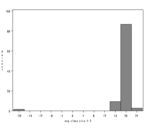
Likewise, a boxplot and stem-and-leaf plot would have called these observations to our attention as well.
In SAS you can use the plot option with proc univariate
to request a boxplot and stem and leaf plot. Below we show just the combined
boxplot and stem and leaf plot from this output. You can see the outlying negative observations way at the bottom of the boxplot.
proc univariate data="c:sasregelemapi" plot;
  var acs_k3;
run;
                      Histogram                       #  Boxplot
     25+*                                              1     0
       .**                                            10     |
       .****************************                 137  +-----+
       .******************************************   207  *--+--*
       .*******                                       34     |
       .*                                              3     0
       .
       .
       .
       .
       .
       .
       .
       .
       .
       .
       .
       .
       .
       .
       .
       .
       .*                                              3     *
    -21+*                                              3     *
        ----+----+----+----+----+----+----+----+--
        * may represent up to 5 counts
We recommend plotting all of these graphs for the variables you will be analyzing. We
will omit, due to space considerations, showing these graphs for all of the variables.
However, in examining the variables, the stem-and-leaf plot for full seemed rather
unusual. Up to now, we have not seen anything problematic with this variable, but
look at the stem and leaf plot for full below. It shows 104 observations where the
percent with a full credential that is much lower than all other
observations. This is over 25% of the schools
and seems very unusual.
proc univariate data="c:sasregelemapi" plot;
  var full;
run;
                   Histogram                   #  Boxplot
  102.5+***************************            81     |
       .******************                     54  +-----+
   92.5+****************                       46  |     |
       .************                           36  *-----*
   82.5+**********                             30  |     |
       .******                                 17  |     |
   72.5+***                                     8  |     |
       .**                                      6  |  +  |
   62.5+**                                      4  |     |
       .**                                      5  |     |
   52.5+*                                       1  |     |
       .**                                      4  |     |
   42.5+*                                       3  |     |
       .*                                       1  |     |
   32.5+                                           |     |
       .                                           |     |
   22.5+                                           |     |
       .                                           |     |
   12.5+                                           |     |
       .                                           |     |
    2.5+***********************************   104  +-----+
        ----+----+----+----+----+----+----+
        * may represent up to 3 counts
Let’s look at the frequency distribution of full to see if we can understand
this better. The values go from 0.42 to 1.0, then jump to 37 and go up from there.
It appears as though some of the percentages are actually entered as proportions,
e.g., 0.42 was entered instead of 42 or 0.96 which really should have been 96.
proc freq data="c:sasregelemapi" ;
  tables full;
run;

                       pct full credential

                                         Cumulative    Cumulative
        full    Frequency     Percent     Frequency      Percent
-----------------------------------------------------------------
0.4199999869           1        0.25             1         0.25
0.4499999881           1        0.25             2         0.50
0.4600000083           1        0.25             3         0.75
0.4699999988           1        0.25             4         1.00
0.4799999893           1        0.25             5         1.25
         0.5           3        0.75             8         2.00
0.5099999905           1        0.25             9         2.25
0.5199999809           1        0.25            10         2.50
0.5299999714           1        0.25            11         2.75
0.5400000215           1        0.25            12         3.00
0.5600000024           2        0.50            14         3.50
0.5699999928           2        0.50            16         4.00
0.5799999833           1        0.25            17         4.25
0.5899999738           3        0.75            20         5.00
0.6000000238           1        0.25            21         5.25
0.6100000143           4        1.00            25         6.25
0.6200000048           2        0.50            27         6.75
0.6299999952           1        0.25            28         7.00
0.6399999857           3        0.75            31         7.75
0.6499999762           3        0.75            34         8.50
0.6600000262           2        0.50            36         9.00
0.6700000167           6        1.50            42        10.50
0.6800000072           2        0.50            44        11.00
0.6899999976           3        0.75            47        11.75
0.6999999881           1        0.25            48        12.00
0.7099999785           1        0.25            49        12.25
0.7200000286           2        0.50            51        12.75
0.7300000191           6        1.50            57        14.25
        0.75           4        1.00            61        15.25
0.7599999905           2        0.50            63        15.75
0.7699999809           2        0.50            65        16.25
0.7900000215           3        0.75            68        17.00
0.8000000119           5        1.25            73        18.25
0.8100000024           8        2.00            81        20.25
0.8199999928           2        0.50            83        20.75
0.8299999833           2        0.50            85        21.25
0.8399999738           2        0.50            87        21.75
0.8500000238           3        0.75            90        22.50
0.8600000143           2        0.50            92        23.00
0.8999999762           3        0.75            95        23.75
0.9200000167           1        0.25            96        24.00
0.9300000072           1        0.25            97        24.25
0.9399999976           2        0.50            99        24.75
0.9499999881           2        0.50           101        25.25
0.9599999785           1        0.25           102        25.50
           1           2        0.50           104        26.00
          37           1        0.25           105        26.25
          41           1        0.25           106        26.50
          44           2        0.50           108        27.00
          45           2        0.50           110        27.50
          46           1        0.25           111        27.75
          48           1        0.25           112        28.00
          53           1        0.25           113        28.25
          57           1        0.25           114        28.50
          58           3        0.75           117        29.25
          59           1        0.25           118        29.50
          61           1        0.25           119        29.75
          63           2        0.50           121        30.25
          64           1        0.25           122        30.50
          65           1        0.25           123        30.75
          68           2        0.50           125        31.25
          69           3        0.75           128        32.00
          70           1        0.25           129        32.25
          71           3        0.75           132        33.00
          72           1        0.25           133        33.25
          73           2        0.50           135        33.75
          74           1        0.25           136        34.00
          75           4        1.00           140        35.00
          76           4        1.00           144        36.00
          77           2        0.50           146        36.50
          78           4        1.00           150        37.50
          79           3        0.75           153        38.25
          80          10        2.50           163        40.75
          81           4        1.00           167        41.75
          82           3        0.75           170        42.50
          83           9        2.25           179        44.75
          84           4        1.00           183        45.75
          85           8        2.00           191        47.75
          86           5        1.25           196        49.00
          87          12        3.00           208        52.00
          88           6        1.50           214        53.50
          89           5        1.25           219        54.75
          90           9        2.25           228        57.00
          91           8        2.00           236        59.00
          92           7        1.75           243        60.75
          93          12        3.00           255        63.75
          94          10        2.50           265        66.25
          95          17        4.25           282        70.50
          96          17        4.25           299        74.75
          97          11        2.75           310        77.50
          98           9        2.25           319        79.75
         100          81       20.25           400       100.00
Let’s see which district(s) these data came from.
proc freq data="c:sasregelemapi" ;
  where (full <= 1);
  tables dnum;
run;
                     district number

                                 Cumulative    Cumulative
dnum    Frequency     Percent     Frequency      Percent
---------------------------------------------------------
 401         104      100.00           104       100.00
We note that all 104 observations in which full was less than or equal to one
came from district 401. Let’s see if this accounts for all of the
observations that come from district 401.
proc freq data="c:sasregelemapi" ;
  where (dnum = 401);
  tables dnum;
run;
                     district number

                                 Cumulative    Cumulative
dnum    Frequency     Percent     Frequency      Percent
---------------------------------------------------------
 401         104      100.00           104       100.00
All of the observations from this district seem to be recorded as proportions instead
of percentages. Again, let us state that this is a pretend problem that we inserted
into the data for illustration purposes. If this were a real life problem, we would
check with the source of the data and verify the problem. We will make a note to fix
this problem in the data as well.
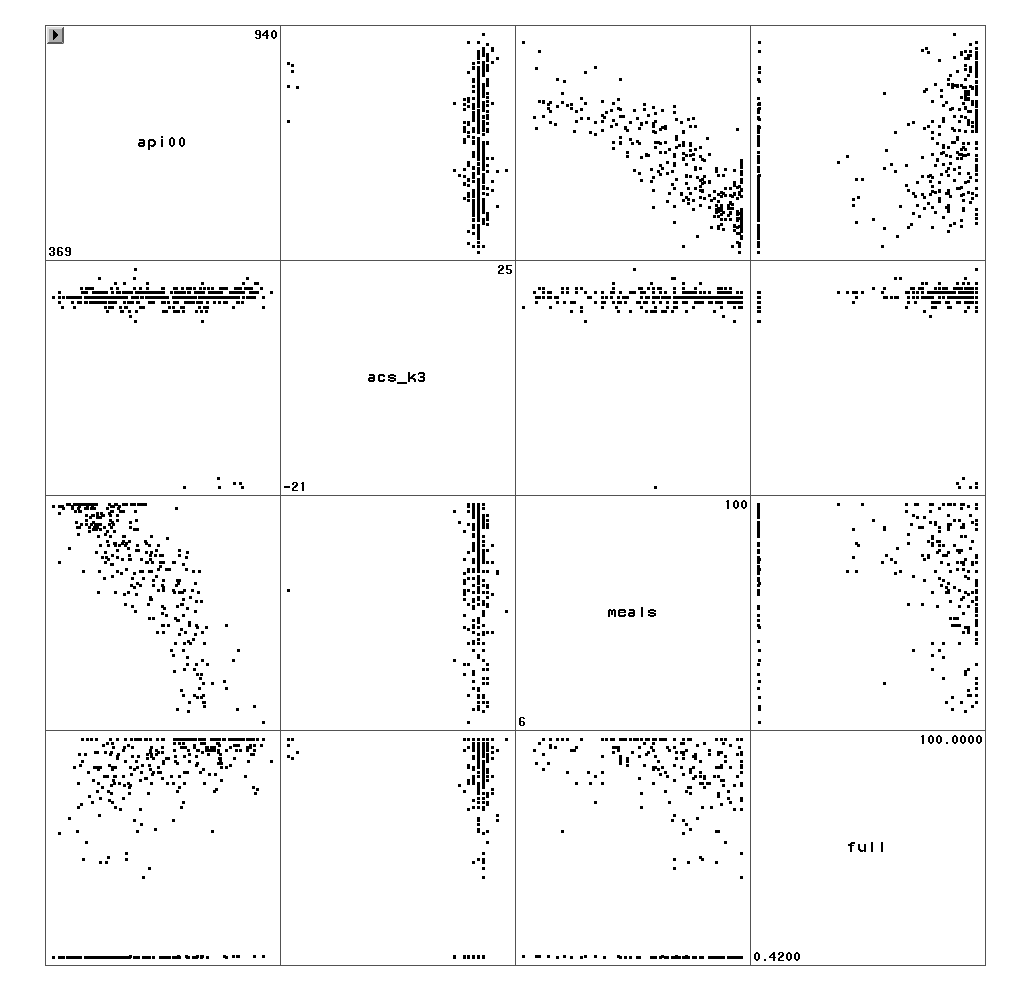
Another useful graphical technique for screening your data is a scatterplot matrix.
While this is probably more relevant as a diagnostic tool searching for non-linearities
and outliers in your data, it can also be a useful data screening tool, possibly revealing
information in the joint distributions of your variables that would not be apparent from
examining univariate distributions. Let’s look at the scatterplot matrix for the
variables in our regression model. This reveals the problems we have already
identified, i.e., the negative class sizes and the percent full credential being entered
as proportions.
proc insight data="c:sasregelemapi";
  scatter api00 acs_k3 meals full *  api00 acs_k3 meals full;
run;
We have identified three problems in our data. There are numerous missing values
for meals, there were negatives accidentally inserted before some of the class
sizes (acs_k3) and over a quarter of the values for full were proportions
instead of percentages. The corrected version of the data is called elemapi2. Let’s use that data file and repeat our analysis and see if the results are the
same as our original analysis. First, let’s repeat our original regression analysis below.
proc reg data="c:sasregelemapi"
  model api00 = acs_k3 meals full;
run;

Dependent Variable: api00 api 2000

                             Analysis of Variance

                                    Sum of           Mean
Source                   DF        Squares         Square    F Value    Pr > F

Model                     3        2634884         878295     213.41    <.0001
Error                   309        1271713     4115.57673
Corrected Total         312        3906597

Root MSE             64.15276    R-Square     0.6745
Dependent Mean      596.40575    Adj R-Sq     0.6713
Coeff Var            10.75656

                                    Parameter Estimates

                                            Parameter       Standard
Variable     Label                  DF       Estimate          Error    t Value    Pr > |t|

Intercept    Intercept               1      906.73916       28.26505      32.08      <.0001
acs_k3       avg class size k-3      1       -2.68151        1.39399      -1.92      0.0553
meals        pct free meals          1       -3.70242        0.15403     -24.04      <.0001
full         pct full credential     1        0.10861        0.09072       1.20      0.2321
Now, let’s use the corrected data file and repeat the regression analysis. We see
quite a difference in the results! In the original analysis (above), acs_k3
was nearly significant, but in the corrected analysis (below) the results show this
variable to be not significant, perhaps due to the cases where class size was given a
negative value. Likewise, the percentage of teachers with full credentials was not
significant in the original analysis, but is significant in the corrected analysis,
perhaps due to the cases where the value was given as the proportion with full credentials
instead of the percent. Also, note that the corrected analysis is based on 398
observations instead of 313 observations, due to getting the complete data for the meals
variable which had lots of missing values.
proc reg data="c:sasregelemapi2";
  model api00 = acs_k3 meals full ;
run;

Dependent Variable: api00 api 2000

                             Analysis of Variance

                                    Sum of           Mean
Source                   DF        Squares         Square    F Value    Pr > F
Model                     3        6604966        2201655     615.55    <.0001
Error                   394        1409241     3576.75370
Corrected Total         397        8014207

Root MSE             59.80597    R-Square     0.8242
Dependent Mean      648.46985    Adj R-Sq     0.8228
Coeff Var             9.22263

                              Parameter Estimates

                                      Parameter     Standard
Variable   Label                DF     Estimate        Error  t Value  Pr > |t|
Intercept  Intercept             1    771.65811     48.86071    15.79    <.0001
acs_k3     avg class size k-3    1     -0.71706      2.23882    -0.32    0.7489
meals      pct free meals        1     -3.68626      0.11178   -32.98    <.0001
full       pct full credential   1      1.32714      0.23887     5.56    <.0001
From this point forward, we will use the corrected, elemapi2, data file.
So far we have covered some topics in data checking/verification, but we have not
really discussed regression analysis itself. Let’s now talk more about performing
regression analysis in SAS.
1.3 Simple Linear Regression
Let’s begin by showing some examples of simple linear regression using SAS. In this
type of regression, we have only one predictor variable. This variable may be continuous,
meaning that it may assume all values within a range, for example, age or height, or it
may be dichotomous, meaning that the variable may assume only one of two values, for
example, 0 or 1. The use of categorical variables with more than two levels will be
covered in Chapter 3. There is only one response or dependent variable, and it is
continuous.
In SAS, the dependent variable is listed immediately after the model
statement followed by an equal sign and then one or more predictor variables. Let’s examine the relationship between the
size of school and academic performance to see if the size of the school is related to
academic performance. For this example, api00 is the dependent variable and enroll
is the predictor.
proc reg data="c:sasregelemapi2";
  model api00 = enroll;
run;
Dependent Variable: api00 api 2000

                             Analysis of Variance

                                    Sum of           Mean
Source                   DF        Squares         Square    F Value    Pr > F
Model                     1         817326         817326      44.83    <.0001
Error                   398        7256346          18232
Corrected Total         399        8073672

Root MSE            135.02601    R-Square     0.1012
Dependent Mean      647.62250    Adj R-Sq     0.0990
Coeff Var            20.84949

                             Parameter Estimates

                                     Parameter     Standard
Variable   Label               DF     Estimate        Error  t Value  Pr > |t|
Intercept  Intercept            1    744.25141     15.93308    46.71    <.0001
enroll     number of students   1     -0.19987      0.02985    -6.70    <.0001
Let’s review this output a bit more carefully. First, we see that the F-test is
statistically significant, which means that the model is statistically significant. The
R-squared is .1012 means that approximately 10% of the variance of api00 is
accounted for by the model, in this case, enroll. The t-test for enroll
equals -6.70 , and is statistically significant, meaning that the regression coefficient
for enroll is significantly different from zero. Note that (-6.70)2 =
44.89, which is the same as the F-statistic (with some rounding error). The coefficient
for enroll is -.19987, or approximately -0.2, meaning that for a one unit increase
in enroll, we would expect a 0.2-unit decrease in api00. In other words,
a school with 1100 students would be expected to have an api score 20 units lower than a
school with 1000 students. The constant is 744.2514, and this is the
predicted value when enroll equals zero. In most cases, the
constant is not very interesting. We have prepared an annotated
output which shows the output from this regression along with an explanation of
each of the items in it.
In addition to getting the regression table, it can be useful to see a scatterplot of
the predicted and outcome variables with the regression line plotted. SAS
makes this very easy for you by using the plot statement as part of proc
reg. For example, below we show how to make a scatterplot of the outcome variable, api00 and the
predictor, enroll. Note that the graph also includes the predicted values
in the form of the regression line.
proc reg data="c:sasregelemapi2";
  model api00 = enroll ;
  plot api00 * enroll ;
run;
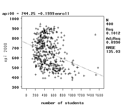
As you see, this one command produces a scatterplot and regression line, and it also
includes the regression model with the correlation of the two variables in the
title. We could include a 95% prediction interval using the pred
option on the plot statement as illustrated below.
proc reg data="c:sasregelemapi2"  ;
  model api00 = enroll ;
  plot api00 * enroll / pred;
run;
quit;
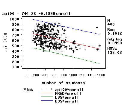
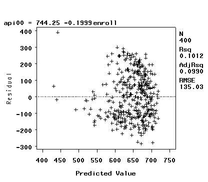
Another kind of graph that you might want to make is a residual versus fitted
plot. As shown below, we can use the plot statement to make this
graph. The keywords residual. and predicted. in this context
refer to the residual value and predicted value from the regression analysis
and can be abbreviated as r. and p. .
proc reg data="c:sasregelemapi2";
  model api00 = enroll ;
  plot residual. * predicted. ;
run;
The table below shows a number of other keywords that can be used with the plot
statement and the statistics they display.
| Keyword | Statistic |
| COOKD. | Cook’s D influence statistics |
| COVRATIO. | standard influence of observation on covariance of betas |
| DFFITS. | standard influence of observation on predicted value |
| H. | leverage |
| LCL. | lower bound of % confidence interval for individual prediction |
| LCLM. | lower bound of % confidence interval for the mean of the dependent variable |
| PREDICTED. | PRED. | P. | predicted values |
| PRESS. | residuals from refitting the model with current observation deleted |
| RESIDUAL. | R. | residuals |
| RSTUDENT. | studentized residuals with the current observation deleted |
| STDI. | standard error of the individual predicted value |
| STDP. | standard error of the mean predicted value |
| STDR. | standard error of the residual |
| STUDENT. | residuals divided by their standard errors |
| UCL. | upper bound of % confidence interval for individual prediction |
| UCLM. | upper bound of % confidence interval for the mean of the dependent variables |
1.4 Multiple Regression
Now, let’s look at an example of multiple regression, in which we have one outcome
(dependent) variable and multiple predictors. For this multiple regression example, we will regress the dependent variable, api00,
on all of the predictor variables in the data set.
proc reg data="c:sasregelemapi2"  ;
  model api00 = ell meals yr_rnd mobility acs_k3 acs_46 full emer enroll ;
run;

Dependent Variable: api00 api 2000

                             Analysis of Variance

                                    Sum of           Mean
Source                   DF        Squares         Square    F Value    Pr > F
Model                     9        6740702         748967     232.41    <.0001
Error                   385        1240708     3222.61761
Corrected Total         394        7981410


Root MSE             56.76810    R-Square     0.8446
Dependent Mean      648.65063    Adj R-Sq     0.8409
Coeff Var             8.75172

                                 Parameter Estimates

                                            Parameter     Standard
Variable   Label                      DF     Estimate        Error  t Value  Pr > |t|
Intercept  Intercept                   1    758.94179     62.28601    12.18    <.0001
ell        english language learners   1     -0.86007      0.21063    -4.08    <.0001
meals      pct free meals              1     -2.94822      0.17035   -17.31    <.0001
yr_rnd     year round school           1    -19.88875      9.25844    -2.15    0.0323
mobility   pct 1st year in school      1     -1.30135      0.43621    -2.98    0.0030
acs_k3     avg class size k-3          1      1.31870      2.25268     0.59    0.5586
acs_46     avg class size 4-6          1      2.03246      0.79832     2.55    0.0113
full       pct full credential         1      0.60972      0.47582     1.28    0.2008
emer       pct emer credential         1     -0.70662      0.60541    -1.17    0.2439
enroll     number of students          1     -0.01216      0.01679    -0.72    0.4693
Let’s examine the output from this regression analysis. As with the simple
regression, we look to the p-value of the F-test to see if the overall model is
significant. With a p-value of zero to four decimal places, the model is statistically
significant. The R-squared is 0.8446, meaning that approximately 84% of the variability of
api00 is accounted for by the variables in the model. In this case, the adjusted
R-squared indicates that about 84% of the variability of api00 is accounted for by
the model, even after taking into account the number of predictor variables in the model.
The coefficients for each of the variables indicates the amount of change one could expect
in api00 given a one-unit change in the value of that variable, given that all
other variables in the model are held constant. For example, consider the variable ell.
We would expect a decrease of 0.86 in the api00 score for every one unit
increase in ell, assuming that all other variables in the model are held
constant. The interpretation of much of the output from the multiple regression is
the same as it was for the simple regression. We have prepared an annotated output that more thoroughly explains the output
of this multiple regression analysis.
You may be wondering what a 0.86 change in ell really means, and how you might
compare the strength of that coefficient to the coefficient for another variable, say meals.
To address this problem, we can use the stb option on the model
statement to request that in addition to the standard output that SAS also
display a table of the standardized values, sometimes called beta
coefficients. Below we show just the portion of the output that includes
these standardized values. The beta coefficients are
used by some researchers to compare the relative strength of the various predictors within
the model. Because the beta coefficients are all measured in standard deviations, instead
of the units of the variables, they can be compared to one another. In other words, the
beta coefficients are the coefficients that you would obtain if the outcome and predictor
variables were all transformed to standard scores, also called z-scores, before running the
regression.
proc reg data="c:sasregelemapi2"  ;
  model api00 = ell meals yr_rnd mobility acs_k3 acs_46 full emer enroll / stb;
run;
                 Parameter Estimates

                                          Standardized
Variable   Label                      DF      Estimate

Intercept  Intercept                   1             0
ell        english language learners   1      -0.14958
meals      pct free meals              1      -0.66070
yr_rnd     year round school           1      -0.05914
mobility   pct 1st year in school      1      -0.06864
acs_k3     avg class size k-3          1       0.01273
acs_46     avg class size 4-6          1       0.05498
full       pct full credential         1       0.06380
emer       pct emer credential         1      -0.05801
enroll     number of students          1      -0.01936
Because these standardized coefficients are all in the same standardized units you
can compare these coefficients to assess the relative strength of each of the
predictors. In this example, meals has the largest Beta coefficient, -0.66,
and acs_k3 has the smallest Beta, 0.013. Thus, a one standard deviation
increase in meals leads to a 0.66 standard deviation decrease in predicted api00,
with the other variables held constant. And, a one standard deviation increase in acs_k3,
in turn, leads to a 0.013 standard deviation increase api00 with the other
variables in the model held constant.
In interpreting this output, remember that the difference between the regular
coefficients (from the prior output) and the standardized coefficients above is
the units of measurement. For example, to
describe the raw coefficient for ell you would say "A one-unit decrease
in ell would yield a .86-unit increase in the predicted api00."
However, for the standardized coefficient (Beta) you would say, "A one standard
deviation decrease in ell would yield a .15 standard deviation increase in the
predicted api00."
So far, we have concerned ourselves with testing a single variable at a time, for
example looking at the coefficient for ell and determining if that is significant.
We can also test sets of variables, using the test command, to see if the set of
variables are significant. First, let’s start by testing a single variable, ell,
using the test statement. Note that the part before the test
command, test1:, is merely a label to identify the output of the test
command. This label could be any short label to identify the output.
proc reg data="c:sasregelemapi2"  ;
  model api00 = ell meals yr_rnd mobility acs_k3 acs_46 full emer enroll ;
  test1: test ell =0;
run;
     Test TEST1 Results for Dependent Variable api00

                                Mean
Source             DF         Square    F Value    Pr > F

Numerator           1          53732      16.67    <.0001
Denominator       385     3222.61761
If you compare this output with the output from the last regression you can see that
the result of the F-test, 16.67, is the same as the square of the result of the t-test in
the regression (-4.083^2 = 16.67). Note that you could get the same results if you typed
the following since SAS defaults to comparing the term(s) listed to 0.
proc reg data="c:sasregelemapi2"  ;
  model api00 = ell meals yr_rnd mobility acs_k3 acs_46 full emer enroll / stb;
  test2: test ell;
run;

     Test TEST2 Results for Dependent Variable api00

                                Mean
Source             DF         Square    F Value    Pr > F

Numerator           1          53732      16.67    <.0001
Denominator       385     3222.61761
Perhaps a more interesting test would be to see if the contribution of class size is
significant. Since the information regarding class size is contained in two
variables, acs_k3 and acs_46, so we include both of these
separated by a comma on the test
command. Below we show just the output from the test command.
proc reg data="c:sasregelemapi2"  ;
  model api00 = ell meals yr_rnd mobility acs_k3 acs_46 full emer enroll ;
  test_class_size: test acs_k3, acs_46;
run;
Test TEST_CLASS_SIZE Results for Dependent Variable api00

                                Mean
Source             DF         Square    F Value    Pr > F

Numerator           2          12742       3.95    0.0200
Denominator       385     3222.61761
The significant F-test, 3.95, means that the collective contribution of these two
variables is significant. One way to think of this, is that there is a significant
difference between a model with acs_k3 and acs_46 as compared to a model
without them, i.e., there is a significant difference between the "full" model
and the "reduced" models.
Finally, as part of doing a multiple regression analysis you might be interested in
seeing the correlations among the variables in the regression model. You can do this
with proc corr as shown below.
proc corr data="c:sasregelemapi2"  ;
  var api00 ell meals yr_rnd mobility acs_k3 acs_46 full emer enroll ;
run;
                            Pearson Correlation Coefficients
                               Prob > |r| under H0: Rho=0
                                  Number of Observations

                                 api00          ell        meals       yr_rnd     mobility

api00                          1.00000     -0.76763     -0.90070     -0.47544     -0.20641
api 2000                                     <.0001       <.0001       <.0001       <.0001
                                   400          400          400          400          399

ell                           -0.76763      1.00000      0.77238      0.49793     -0.02046
english language learners       <.0001                    <.0001       <.0001       0.6837
                                   400          400          400          400          399

meals                         -0.90070      0.77238      1.00000      0.41845      0.21665
pct free meals                  <.0001       <.0001                    <.0001       <.0001
                                   400          400          400          400          399

yr_rnd                        -0.47544      0.49793      0.41845      1.00000      0.03479
year round school               <.0001       <.0001       <.0001                    0.4883
                                   400          400          400          400          399

mobility                      -0.20641     -0.02046      0.21665      0.03479      1.00000
pct 1st year in school          <.0001       0.6837       <.0001       0.4883
                                   399          399          399          399          399

acs_k3                         0.17100     -0.05565     -0.18797      0.02270      0.04014
avg class size k-3              0.0006       0.2680       0.0002       0.6517       0.4245
                                   398          398          398          398          398

acs_46                         0.23291     -0.17330     -0.21309     -0.04207      0.12769
avg class size 4-6              <.0001       0.0005       <.0001       0.4032       0.0110
                                   397          397          397          397          396

full                           0.57441     -0.48476     -0.52756     -0.39771      0.02521
pct full credential             <.0001       <.0001       <.0001       <.0001       0.6156
                                   400          400          400          400          399

emer                          -0.58273      0.47218      0.53304      0.43472      0.05961
pct emer credential             <.0001       <.0001       <.0001       <.0001       0.2348
                                   400          400          400          400          399

enroll                        -0.31817      0.40302      0.24103      0.59182      0.10502
number of students              <.0001       <.0001       <.0001       <.0001       0.0360
                                   400          400          400          400          399

                            Pearson Correlation Coefficients
                               Prob > |r| under H0: Rho=0
                                  Number of Observations

                                acs_k3       acs_46         full         emer       enroll

api00                          0.17100      0.23291      0.57441     -0.58273     -0.31817
api 2000                        0.0006       <.0001       <.0001       <.0001       <.0001
                                   398          397          400          400          400

ell                           -0.05565     -0.17330     -0.48476      0.47218      0.40302
english language learners       0.2680       0.0005       <.0001       <.0001       <.0001
                                   398          397          400          400          400

meals                         -0.18797     -0.21309     -0.52756      0.53304      0.24103
pct free meals                  0.0002       <.0001       <.0001       <.0001       <.0001
                                   398          397          400          400          400

yr_rnd                         0.02270     -0.04207     -0.39771      0.43472      0.59182
year round school               0.6517       0.4032       <.0001       <.0001       <.0001
                                   398          397          400          400          400

mobility                       0.04014      0.12769      0.02521      0.05961      0.10502
pct 1st year in school          0.4245       0.0110       0.6156       0.2348       0.0360
                                   398          396          399          399          399

acs_k3                         1.00000      0.27078      0.16057     -0.11033      0.10890
avg class size k-3                           <.0001       0.0013       0.0277       0.0298
                                   398          395          398          398          398

acs_46                         0.27078      1.00000      0.11773     -0.12446      0.02829
avg class size 4-6              <.0001                    0.0190       0.0131       0.5741
                                   395          397          397          397          397

full                           0.16057      0.11773      1.00000     -0.90568     -0.33769
pct full credential             0.0013       0.0190                    <.0001       <.0001
                                   398          397          400          400          400

emer                          -0.11033     -0.12446     -0.90568      1.00000      0.34309
pct emer credential             0.0277       0.0131       <.0001                    <.0001
                                   398          397          400          400          400

enroll                         0.10890      0.02829     -0.33769      0.34309      1.00000
number of students              0.0298       0.5741       <.0001       <.0001
                                   398          397          400          400          400
We can see that the strongest correlation with api00 is meals
with a correlation in excess of -0.9. The variables ell and emer
are also strongly correlated with api00.
All three of these correlations are negative, meaning that as the value of one variable
goes down, the value of the other variable tends to go up. Knowing that these variables
are strongly associated with api00, we might predict that they would be
statistically significant predictor variables in the regression model. Note that
the number of cases used for each correlation is determined on a
"pairwise" basis, for example there are 398 valid pairs of data for enroll
and acs_k3, so that correlation of .1089 is based on 398 observations.
1.5 Transforming Variables
Earlier we focused on screening your data for potential errors. In the next
chapter, we will focus on regression diagnostics to verify whether your data meet the
assumptions of linear regression. Here, we will focus on the issue
of normality. Some researchers believe that linear regression requires that the outcome (dependent)
and predictor variables be normally distributed. We need to clarify this issue. In
actuality, it is the residuals that need to be normally distributed. In fact,
the residuals need to be normal only for the t-tests to be valid. The estimation of the
regression coefficients do not require normally distributed residuals. As we are
interested in having valid t-tests, we will investigate issues concerning normality.
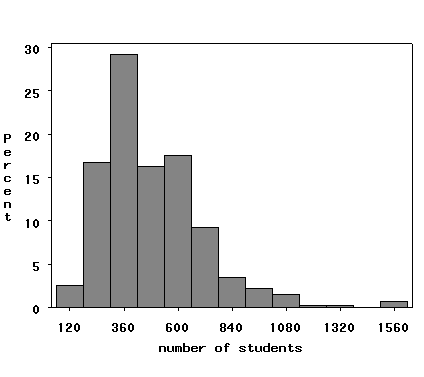
A common cause of non-normally distributed residuals is non-normally distributed
outcome and/or predictor variables. So, let us explore the distribution of our
variables and how we might transform them to a more normal shape. Let’s start by
making a histogram of the variable enroll, which we looked at earlier in the simple
regression.
proc univariate data="c:sasregelemapi2";
  var enroll ;
  histogram / cfill=gray;
run;
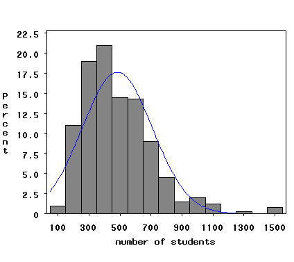
We can use the normal option to superimpose a normal curve on this graph and the
midpoints option to indicate that we want bins with midpoints from 100 to
1500 going in increments of 100.
proc univariate data="c:sasregelemapi2";
  var enroll ;
  histogram / cfill=gray normal midpoints=100 to 1500 by 100;
run;
Histograms are sensitive to the number of bins or columns that are used in the display.
An alternative to histograms is the kernel density plot, which approximates the
probability density of the variable. Kernel density plots have the advantage of being
smooth and of being independent of the choice of origin, unlike histograms. You
can add a kernel density plot to the above plot with he kernel option as
illustrated below.
proc univariate data="c:sasregelemapi2";
  var enroll ;
  histogram / cfill=gray normal midpoints=100 to 1500 by 100 kernel;
run;
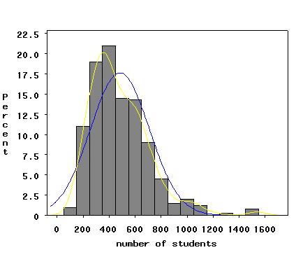
Not surprisingly, the kdensity plot also indicates that the variable enroll
does not look normal.
There are two other types of graphs that are often used to examine the distribution
of variables; quantile-quantile plots and normal probability plots.
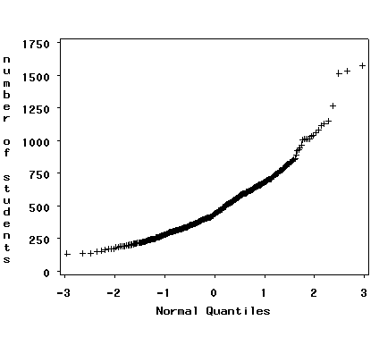
A quantile-quantile plot graphs the quantiles of a variable against the quantiles of a
normal (Gaussian) distribution. Such plots are sensitive to non-normality near the tails,
and indeed we see considerable deviations from normal, the diagonal line, in the tails.
This plot is typical of variables that are strongly skewed to the right.
proc univariate data="c:sasregelemapi2";
  var enroll ;
  qqplot / normal;
run;
The normal probability plot is also useful for examining the distribution of
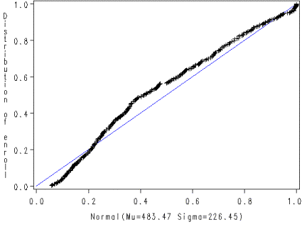
variables and is sensitive to deviations from normality nearer to
the center of the distribution. We will use SAS proc capability to get the
normal probability plot. Again, we see indications non-normality in enroll.
proc capability data="c:sasregelemapi2" noprint;
  ppplot enroll ;
run;
Given the skewness to the right in enroll, let us try a log
transformation to see if that makes it more normal. Below we create a
variable lenroll that is the natural log of enroll and then we
repeat some of the above commands to see if lenroll is more normally
distributed.
data elemapi3;
  set "c:sasregelemapi2";
  lenroll = log(enroll);
run;
Now let’s try showing a histogram for lenroll with a normal overlay
and a kernel density estimate.
proc univariate data=elemapi3 noprint;
  var lenroll ;
  histogram / cfill=grayd0  normal kernel (color = red);
run;
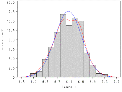
We can see that lenroll looks quite normal. We could then create
a quantile-quantile plot and a normal probability plot to further assess whether lenroll seems
normal, as well as seeing how lenroll impacts the residuals, which is really the
important consideration.
1.6 Summary
In this lecture we have discussed the basics of how to perform simple and multiple
regressions, the basics of interpreting output, as well as some related commands. We
examined some tools and techniques for screening for bad data and the consequences such
data can have on your results. Finally, we touched on the assumptions of linear
regression and illustrated how you can check the normality of your variables and how you
can transform your variables to achieve normality. The next chapter will pick up
where this chapter has left off, going into a more thorough discussion of the assumptions
of linear regression and how you can use SAS to assess these assumptions for your data.
In particular, the next lecture will address the following issues.
- Checking for points that exert undue influence on the coefficients
- Checking for constant error variance (homoscedasticity)
- Checking for linear relationships
- Checking model specification
- Checking for multicollinearity
- Checking normality of residuals
1.7 For more information
- Related Web Pages