Power Analysis for Paired Sample t-test

Examples

Example 1. A company markets an eight week long weight loss program and claims that at the end of the program on average a participant will have lost 5 pounds. On the other hand, you have studied the program and you believe that their program is scientifically unsound and shouldn’t work at all. With some limited funding at hand, you want test the hypothesis that the weight loss program does not help people lose weight. Your plan is to get a random sample of people and put them on the program. You will measure their weight at the beginning of the program and then measure their weight again at the end of the program.  Based on some previous research, you believe that the standard deviation of the weight difference over eight weeks will be 5 pounds. You now want to know how many people you should enroll in the program to test your hypothesis.

Example 2. A human factors researcher wants to study the difference between dominant hand and the non-dominant hand in terms of manual dexterity. She designs an experiment where each subject would place 10 small beads on the table in a bowl, once with the dominant hand and once with the non-dominant hand. She measured the number seconds needed in each round to complete the task. She has also decided that the order in which the two hands are measured should be counter balanced. She expects that the average difference in time would be 5 seconds with the dominant hand being more efficient with standard deviation of 10. She collects her data on a sample of 35 subjects. The question is, what is the statistical power of her design with an N of 35 to detect the difference in the magnitude of 5 seconds.

Prelude to the Power Analysis

In both of the examples, there are two measures on each subject, and we are interested in the mean of the difference of the two measures. This can be done with a t-test for paired samples (dependent samples). In a power analysis, there are always a pair of hypotheses:  a specific null hypothesis and a specific alternative hypothesis. For instance, in Example 1, the null hypothesis is that the mean weight loss is 5 pounds and the alternative is zero pounds. In Example 2, the null hypothesis is that mean difference is zero seconds and the alternative hypothesis is that the mean difference is 5 seconds.

There are two different aspects of power analysis. One is to calculate the necessary sample size for a specified power. The other aspect is to calculate the power when given a specific sample size. Technically, power is the probability of rejecting the null hypothesis when the specific alternative hypothesis is true.

Both of these calculations depend on the Type I error rate, the significance level. The significance level (called alpha), or the Type I error rate, is the probability of rejecting H₀ when it is actually true. The smaller the Type I error rate, the larger the sample size required for the same power. Likewise, the smaller the Type I error rate, the smaller the power for the same sample size. This is the trade-off between the reliability and sensitivity of the test.

Power Analysis

In SPSS, it is fairly straightforward to perform a power analysis for the paired sample t-test using SPSS’s power means related command.

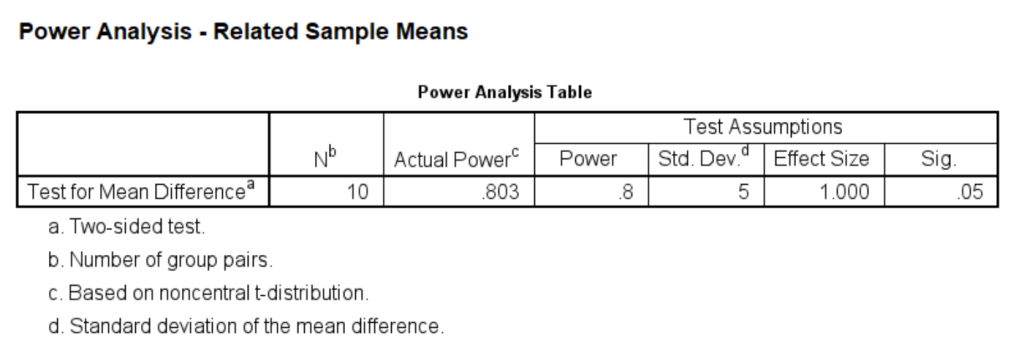
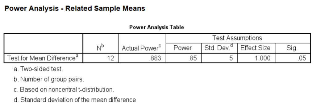
For the calculation of Example 1, we can set the power at different levels and calculate the sample size for each level. For example, we can set the power to be at the .80 level at first, and then reset it to be at the .85 level, and so on.

power means related 
  /parameters test=nondirectional significance=0.05 power=.8 sd=5 mean=5.

power means related 
  /parameters test=nondirectional significance=0.05 power=.85 sd=5 mean=5.

power means related 
  /parameters test=nondirectional significance=0.05 power=.9 sd=5 mean=5.

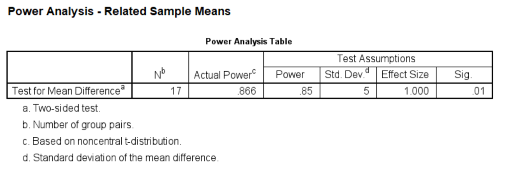
Next, let’s change the level of significance to .01 with a power of .85. What does this mean for our sample size calculation?

power means related 
  /parameters test=nondirectional significance=0.01 power=.85 sd=5 mean=5.

As you can see, the sample size goes up from 13 to 17 for specified power of .85 when alpha drops from .05 to .01.

This means if we want our test to be more reliable, i.e., not rejecting the null hypothesis in case it is true, we will need a larger sample size. If we think that we want a lower alpha at 0.01 level and a high power at .90, then we would need 19 subjects as shown below. Remember this is under the normality assumption. If the distribution is not normal, then 19 subjects are, in general, not enough for this t-test.

power means related 
  /parameters test=nondirectional power=.90 significance=.01 sd=5 mean=5.

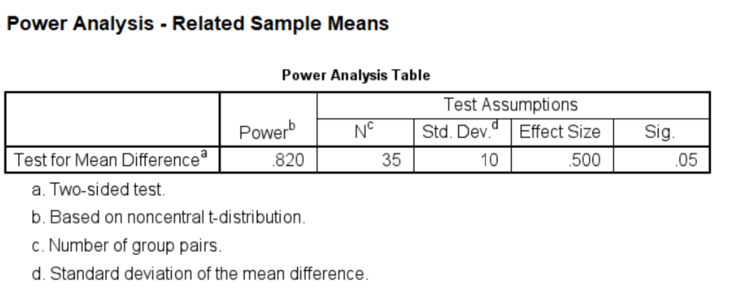
Now, let’s now turn our calculation around the other way. Let’s look at Example 2. In this example, our researcher has already collected data on 35 subjects. How much statistical power does her design have to detect the difference of 5 seconds with standard deviation of 10 seconds?

Again we use the power means related command to calculate the power.

power means related 
  /parameters test=nondirectional significance=0.05 npairs=35 sd=10 mean=0 5.

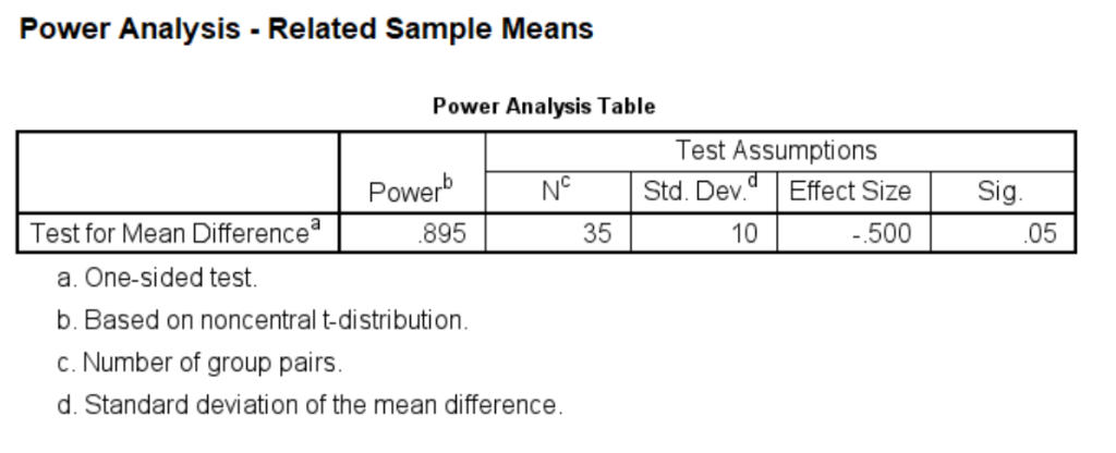
This means that the researcher would detect the difference of 5 seconds about 82 percent of the time.  Notice we did this as two-sided test. Since it is believed that our dominant hand is always better than the non-dominant hand, the researcher actually could conduct a one-tailed test. Now, let’s recalculate the power for one-tailed paired-sample t-test.

power means related 
  /parameters test=directional significance=0.05 npairs=35 sd=10 mean=0 5.

Discussion

You have probably noticed that the way to conduct the power analysis for paired-sample t-test is the same as for the one-sample t-test. This is due to the fact that in the paired-sample t-test we compute the difference in the two scores for each subject and then compute the mean and standard deviation of the differences. This turns the paired-sample t-test into a one-sample t-test.

The other technical assumption is the normality assumption. If the distribution is skewed, then a small sample size may not have the power shown in the results, because the value in the results is calculated using the method based on the normality assumption. It might not even be a good idea to do a t-test on a small sample to begin with.

What we really need to know is the difference between the two means, not the individual values. In fact, what really matters, is the difference of the means over the standard deviation. We call this the effect size. It is usually not an easy task to determine the effect size. It usually comes from studying the existing literature or from pilot studies. A good estimate of the effect size is the key to a successful power analysis.

See Also

• References
  • D. Moore and G. McCabe, Introduction to the Practice
  of Statistics, Third Edition, Section 6.4.