Examples
Example 1. A company that manufactures light bulbs claims that a particular type of light bulb will last 850 hours on average with standard deviation of 50. A consumer protection group thinks that the manufacturer has overestimated the lifespan of their light bulbs by about 40 hours. How many light bulbs does the consumer protection group have to test in order to prove their point with reasonable confidence?
Example 2. It has been estimated that the average height of American white male adults is 70 inches. It has also been postulated that there is a positive correlation between height and intelligence. If this is true, then the average height of a white male graduate students on campus should be greater than the average height of American white male adults in general. You want to test this theory out by random sampling a small group of white male graduate students. But you need to know how small the group can be or how few people that you need to measure such that you can still prove your point.
Prelude to the Power Analysis
For the power analysis below, we are going to focus on Example 1, testing the average lifespan of a light bulb. Our first goal is to figure out the number of light bulbs that need to be tested. That is, we will determine the sample size for a given a significance level and power. Next, we will reverse the process and determine the power, given the sample size and the significance level.
We know so far that the manufacturer claims that the average lifespan of the light bulb is 850 with the standard deviation of 50, and the consumer protection group believes that the manufacturer has overestimated by about 40 hours. So in terms of hypotheses, our null hypothesis is H0 = 850 and our alternative hypothesis is Ha= 810.
The significance level is the probability of a Type I error, that is the probability of rejecting H0 when it is actually true. We will set it at the .05 level. The power of the test against Ha is the probability of that the test rejects H0. We will set it at .90 level.
We are almost ready for our power analysis. But let’s talk about the standard deviation a little bit. Intuitively, the number of light bulbs we need to test depends on the variability of the lifespan of these light bulbs. Take an extreme case where all the light bulbs have exactly the same lifespan. Then we just need to check a single light bulb to prove our point. Of course, this will never happen. On the other hand, suppose that some light bulbs last for 1000 hours and some only last 500 hours. We will have to select quite a few of light bulbs to cover all the ground. Therefore, the standard deviation for the distribution of the lifespan of the light bulbs will play an important role in determining the sample size.
Power Analysis
In SPSS, it is fairly straightforward to perform a power analysis for comparing means. For example, we can use SPSS’s power mean onesample command for our calculation as shown below using the information we discussed above.
power means onesample
  /parameters test=nondirectional significance=0.05 power=0.9 sd=50 mean=850 null=810.
The result tells us that we need a sample size at least 19 light bulbs to reject H0 under the alternative hypothesis Ha to have a power of 0.9.
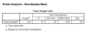
Next, suppose we have a sample of size 10. How much power do we have keeping all of the other numbers the same? We can use the same command, power means onesample, to calculate it.
power means onesample
  /parameters test=nondirectional significance=0.05 n=10 sd=50 mean=850 null=810.
You can see that the power is about .62 for a sample size of 10.
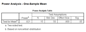
What then is the power for sample size of 15?
power means onesample
  /parameters test=nondirectional significance=0.05 n=15 sd=50 mean=850 null=810.
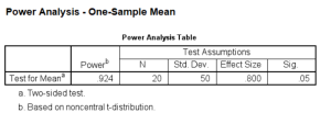
So now the power is about .82. You could also do it again to find out the power for a sample size of 20. You’ll probably expect that the power will be greater.
power means onesample
  /parameters test=nondirectional significance=0.05 n=20 sd=50 mean=850 null=810.
We can also expect that if we specified a lower power or the standard deviation is smaller, then the sample size should also be smaller. We can experiment with different values of power and standard deviation as shown below.
power means onesample
  /parameters test=nondirectional significance=0.05 power=0.8 sd=50 mean=850 null=810.
If the standard deviation is lower, then the sample size should also go down, as we discussed before.
power means onesample
  /parameters test=nondirectional significance=0.05 power=0.8 sd=30 mean=850 null=810.
Discussion
There is another technical assumption, the normality assumption. If the variable is not normally distributed, a small sample size usually will not have the power indicated in the results, because those results are calculated using the common method based on the normality assumption. It might not even be a good idea to do a t-test on such a small sample to begin with if the normality assumption is in question.
Here is another technical point. What we really need to know is the difference between the two means, not the individual values. In fact, what really matters is the difference of the means over the standard deviation. We call this the effect size. For example, we would get the same power if we subtracted 800 from each mean, changing 850 to 50 and 810 to 10.
power means onesample
  /parameters test=nondirectional significance=0.05 power=0.8 sd=50 mean=50 null=10.
If we standardize our variable, we can calculate the means in terms of change in standard deviations.
power means onesample
  /parameters test=nondirectional significance=0.05 power=0.8 sd=1 mean=1 null=0.2.
It is usually not an easy task to determine the “true” effect size. We make our best guess based upon the existing literature, a pilot study or the smallest effect size of interest. A good estimate of the effect size is the key to a successful power analysis.
See Also
D. Moore and G. McCabe, Introduction to the Practice of Statistics, Third Edition, Section 6.4.


