Table 11.1, page 360 and Figure 11.1, page 359
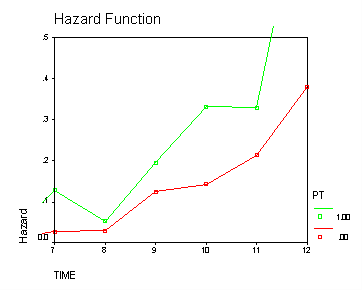
The code below produces the top two panels of the table. The plot subcommands produce the graphs shown in Figure 11.1. Note that the values shown in the last line in each panel is different from those shown in the text. We believe that this is because SPSS uses a different algorithm. Hence, the last point in each graph is also different from that shown in the text. Also note that on the interval subcommand we go through 13 instead of 12. This is so that the graph goes through 12.
get file 'c:aldafirstsex.sav'.

survival table = time by pt(0 1)
 /interval = thru 13 by 1
 /status = censor(0)
 /plot hazard survival.
This subfile contains:     180 observations

 Life Table
   Survival Variable  TIME
                 for  PT
                                                  =       0

        Number  Number  Number  Number                  Cumul
Intrvl  Entrng  Wdrawn  Exposd    of    Propn   Propn   Propn   Proba-
Start    this   During    to    Termnl  Termi-  Sur-    Surv    bility  Hazard
Time    Intrvl  Intrvl   Risk   Events  nating  viving  at End  Densty   Rate
------  ------  ------  ------  ------  ------  ------  ------  ------  ------
    .0    72.0      .0    72.0      .0   .0000  1.0000  1.0000   .0000   .0000
   1.0    72.0      .0    72.0      .0   .0000  1.0000  1.0000   .0000   .0000
   2.0    72.0      .0    72.0      .0   .0000  1.0000  1.0000   .0000   .0000
   3.0    72.0      .0    72.0      .0   .0000  1.0000  1.0000   .0000   .0000
   4.0    72.0      .0    72.0      .0   .0000  1.0000  1.0000   .0000   .0000
   5.0    72.0      .0    72.0      .0   .0000  1.0000  1.0000   .0000   .0000
   6.0    72.0      .0    72.0      .0   .0000  1.0000  1.0000   .0000   .0000
   7.0    72.0      .0    72.0     2.0   .0278   .9722   .9722   .0278   .0282
   8.0    70.0      .0    70.0     2.0   .0286   .9714   .9444   .0278   .0290
   9.0    68.0      .0    68.0     8.0   .1176   .8824   .8333   .1111   .1250
  10.0    60.0      .0    60.0     8.0   .1333   .8667   .7222   .1111   .1429
  11.0    52.0      .0    52.0    10.0   .1923   .8077   .5833   .1389   .2128
  12.0+   42.0    34.0    25.0     8.0   .3200   .6800   .3967     **      **

 **     These calculations for the last interval are meaningless.

 The median survival time for these data is  12.00+

 Life Table
   Survival Variable  TIME
                 for  PT
                                                  =       1

        Number  Number  Number  Number                  Cumul
Intrvl  Entrng  Wdrawn  Exposd    of    Propn   Propn   Propn   Proba-
Start    this   During    to    Termnl  Termi-  Sur-    Surv    bility  Hazard
Time    Intrvl  Intrvl   Risk   Events  nating  viving  at End  Densty   Rate
------  ------  ------  ------  ------  ------  ------  ------  ------  ------
    .0   108.0      .0   108.0      .0   .0000  1.0000  1.0000   .0000   .0000
   1.0   108.0      .0   108.0      .0   .0000  1.0000  1.0000   .0000   .0000
   2.0   108.0      .0   108.0      .0   .0000  1.0000  1.0000   .0000   .0000
   3.0   108.0      .0   108.0      .0   .0000  1.0000  1.0000   .0000   .0000
   4.0   108.0      .0   108.0      .0   .0000  1.0000  1.0000   .0000   .0000
   5.0   108.0      .0   108.0      .0   .0000  1.0000  1.0000   .0000   .0000
   6.0   108.0      .0   108.0      .0   .0000  1.0000  1.0000   .0000   .0000
   7.0   108.0      .0   108.0    13.0   .1204   .8796   .8796   .1204   .1281
   8.0    95.0      .0    95.0     5.0   .0526   .9474   .8333   .0463   .0541
   9.0    90.0      .0    90.0    16.0   .1778   .8222   .6852   .1481   .1951
  10.0    74.0      .0    74.0    21.0   .2838   .7162   .4907   .1944   .3307
  11.0    53.0      .0    53.0    15.0   .2830   .7170   .3519   .1389   .3297
  12.0+   38.0    20.0    28.0    18.0   .6429   .3571   .1257     **      **

 **     These calculations for the last interval are meaningless.
The code below produces the bottom panel of the table.
survival table = time
 /interval = thru 12 by 1
 /status = censor(0).
This subfile contains:     180 observations

 Life Table
   Survival Variable  TIME

        Number  Number  Number  Number                  Cumul
Intrvl  Entrng  Wdrawn  Exposd    of    Propn   Propn   Propn   Proba-
Start    this   During    to    Termnl  Termi-  Sur-    Surv    bility  Hazard
Time    Intrvl  Intrvl   Risk   Events  nating  viving  at End  Densty   Rate
------  ------  ------  ------  ------  ------  ------  ------  ------  ------
    .0   180.0      .0   180.0      .0   .0000  1.0000  1.0000   .0000   .0000
   1.0   180.0      .0   180.0      .0   .0000  1.0000  1.0000   .0000   .0000
   2.0   180.0      .0   180.0      .0   .0000  1.0000  1.0000   .0000   .0000
   3.0   180.0      .0   180.0      .0   .0000  1.0000  1.0000   .0000   .0000
   4.0   180.0      .0   180.0      .0   .0000  1.0000  1.0000   .0000   .0000
   5.0   180.0      .0   180.0      .0   .0000  1.0000  1.0000   .0000   .0000
   6.0   180.0      .0   180.0      .0   .0000  1.0000  1.0000   .0000   .0000
   7.0   180.0      .0   180.0    15.0   .0833   .9167   .9167   .0833   .0870
   8.0   165.0      .0   165.0     7.0   .0424   .9576   .8778   .0389   .0433
   9.0   158.0      .0   158.0    24.0   .1519   .8481   .7444   .1333   .1644
  10.0   134.0      .0   134.0    29.0   .2164   .7836   .5833   .1611   .2427
  11.0   105.0      .0   105.0    25.0   .2381   .7619   .4444   .1389   .2703
  12.0+   80.0    54.0    53.0    26.0   .4906   .5094   .2264     **      **

 **     These calculations for the last interval are meaningless.
Figure 11.1, page 359
Top panel:
The plots shown below were created by the /plots subcommand in the survival command. We modified each graph by double clicking on it (to open the Chart Editor), and then double clicking on the axes to adjust the minimum, maximum and increment values. We clicked on the Format tab at the top of the Chart Editor and selected Interpolation to change the way the dots were connected to "straight" and then clicked on "Apply All" to apply this style of connection to both lines.
Bottom panel:
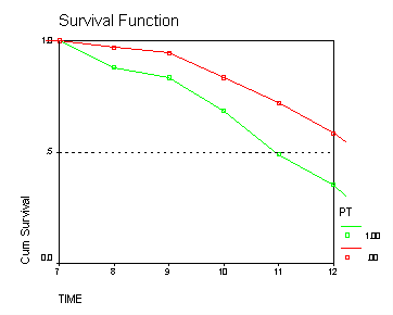
Figure 11.2, page 363
Top panel: This is the same as the hazard shown above.
Middle panel:
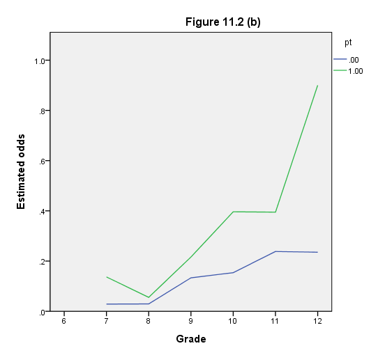
Before we can create the graph, we need to run two logistic regressions, one for each value of pt. An easy way to do this in SPSS is to split the data file into two parts, one for each value of pt. To do this, we first sort the data on pt and then use the temporary command so that the splitting of the data file is not permanent. We use the save subcommand in the logistic command to save the predicted values, which we call pred (the name of the variable containing the predicted values is in parentheses). We use the compute command to calculate the odds that we need for the graph. Finally, we use the ggraph command to create the graph.
get file 'c:aldafirstsex_pp.sav'.
sort cases by pt.
temporary.
split file by pt.
logistic regression var = event
 /method = enter d7 to d12
 /origin
 /save pred (pred).

compute odds = pred/(1-pred).
execute.
formats odds (f3.1) period (f2.0).
GGRAPH
  /GRAPHDATASET NAME="iGraphDataset" VARIABLES= odds period pt
  /GRAPHSPEC SOURCE=INLINE .
BEGIN GPL
SOURCE: s=userSource( id( "iGraphDataset" ) )
DATA: odds=col( source(s), name( "odds" ) )
DATA: period=col( source(s), name( "period" ) )
DATA: pt=col( source(s), name( "pt" ), unit.category()  )
GUIDE: text.title( label( "Figure 11.2 (b)" ) )
GUIDE: axis( dim( 1 ), label( "Grade" ) )
GUIDE: axis( dim( 2 ), label( "Estimated odds" ) )
GUIDE: legend( aesthetic( aesthetic.color ), label( "pt" ) )
GUIDE: legend( aesthetic( aesthetic.color.exterior ), label( "pt" ) )
SCALE: linear( dim( 1 ), min( 6 ), max( 12 ) )
SCALE: linear( dim( 2 ), min( 0 ), max( 1 ) )
ELEMENT: line( position( summary.mean( period * odds ) ), color( pt )  )
END GPL.
Bottom panel:
compute logit = ln(odds).
execute.
formats logit (f4.1).
GGRAPH
  /GRAPHDATASET NAME="iGraphDataset" VARIABLES= logit period pt
  /GRAPHSPEC SOURCE=INLINE .
BEGIN GPL
SOURCE: s=userSource( id( "iGraphDataset" ) )
DATA: logit=col( source(s), name( "logit" ) )
DATA: period=col( source(s), name( "period" ) )
DATA: pt=col( source(s), name( "pt" ), unit.category()  )
GUIDE: text.title( label( "Figure 11.2 (c)" ) )
GUIDE: axis( dim( 1 ), label( "Grade" ) )
GUIDE: axis( dim( 2 ), label( "Estimated logit(hazard)" ) )
GUIDE: legend( aesthetic( aesthetic.color ), label( "pt" ) )
GUIDE: legend( aesthetic( aesthetic.color.exterior ), label( "pt" ) )
SCALE: linear( dim( 1 ), min( 6 ), max( 12 ) )
SCALE: linear( dim( 2 ), min( -4 ), max( 0 ) )
ELEMENT: line( position( summary.mean( period * logit ) ), color( pt ) )
END GPL.
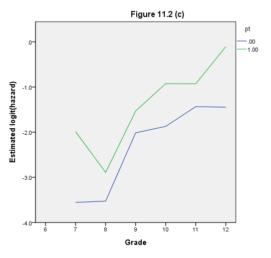
Figure 11.3, page 366
get file 'c:aldafirstsex_pp.sav'.

sort cases by period pt event.

aggregate outfile = * mode = addvariables
/break= period pt
/c1 = nu(id).

aggregate outfile = * mode = addvariables
/break= period pt event
/c2 = nu(id).

compute prob = c2/c1.
if event = 1 & pt = 0 pt0 = ln(prob/(1 - prob)).
if event = 1 & pt = 1 pt1 = ln(prob/(1 - prob)).
compute pt01 = pt0.
if sysmis(pt0) pt01 = pt1.
exe.

logistic regression var = event
/method = enter pt
/save = pred(p1).

compute lp1 = ln(p1/(1 - p1)).
sort cases by pt period.
exe.

formats pt01 lp1 (f3.1) period (f2.0).
GGRAPH
  /GRAPHDATASET NAME="iGraphDataset" VARIABLES= pt01 lp1 period pt
  /GRAPHSPEC SOURCE=INLINE .
BEGIN GPL
SOURCE: s=userSource( id( "iGraphDataset" ) )
DATA: pt01=col( source(s), name( "pt01" ) )
DATA: lp1=col( source(s), name( "lp1" ) )
DATA: period=col( source(s), name( "period" ) )
DATA: pt=col( source(s), name( "pt" ), unit.category()  )
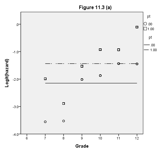
GUIDE: text.title( label( "Figure 11.3 (a)" ) )
GUIDE: axis( dim( 1 ), label( "Grade" ) )
GUIDE: axis( dim( 2 ), label( "Logit(hazard)" ) )
GUIDE: legend( aesthetic( aesthetic.shape ), label( "pt" ) )
GUIDE: legend( aesthetic( aesthetic.shape.exterior ), label( "pt" ) )
SCALE: linear( dim( 1 ), min( 6 ), max( 12 ) )
SCALE: linear( dim( 2 ), min( -4 ), max( 0 ) )
ELEMENT: point( position( period * pt01 ), shape(pt)  )
ELEMENT: line( position( ( period * lp1 ) ), shape( pt )  )
END GPL.
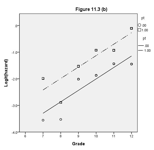
* panel b.

logistic regression var = event
/method = enter period pt
/save pred (p2).

compute lp2 = ln(p2/(1 - p2)).
exe.

formats lp2 (f3.1).
GGRAPH
  /GRAPHDATASET NAME="iGraphDataset" VARIABLES= pt01 lp2 period pt
  /GRAPHSPEC SOURCE=INLINE .
BEGIN GPL
SOURCE: s=userSource( id( "iGraphDataset" ) )
DATA: pt01=col( source(s), name( "pt01" ) )
DATA: lp2=col( source(s), name( "lp2" ) )
DATA: period=col( source(s), name( "period" ) )
DATA: pt=col( source(s), name( "pt" ), unit.category()  )
GUIDE: text.title( label( "Figure 11.3 (b)" ) )
GUIDE: axis( dim( 1 ), label( "Grade" ) )
GUIDE: axis( dim( 2 ), label( "Logit(hazard)" ) )
GUIDE: legend( aesthetic( aesthetic.shape ), label( "pt" ) )
GUIDE: legend( aesthetic( aesthetic.shape.exterior ), label( "pt" ) )
SCALE: linear( dim( 1 ), min( 6 ), max( 12 ) )
SCALE: linear( dim( 2 ), min( -4 ), max( 0 ) )
ELEMENT: point( position( period * pt01 ), shape(pt)  )
ELEMENT: line( position( ( period * lp2 ) ), shape( pt )  )
END GPL.
* panel c.

logistic regression var = event
/method = enter d7 d8 d9 d10 d11 d12 pt
/origin
/save pred (p3).

compute lp3 = ln(p3/(1 - p3)).
exe.

formats lp3 (f3.1).
GGRAPH
  /GRAPHDATASET NAME="iGraphDataset" VARIABLES= pt01 lp3 period pt
  /GRAPHSPEC SOURCE=INLINE .
BEGIN GPL
SOURCE: s=userSource( id( "iGraphDataset" ) )
DATA: pt01=col( source(s), name( "pt01" ) )
DATA: lp3=col( source(s), name( "lp3" ) )
DATA: period=col( source(s), name( "period" ) )
DATA: pt=col( source(s), name( "pt" ), unit.category()  )
GUIDE: text.title( label( "Figure 11.3 (c)" ) )
GUIDE: axis( dim( 1 ), label( "Grade" ) )
GUIDE: axis( dim( 2 ), label( "Logit(hazard)" ) )
GUIDE: legend( aesthetic( aesthetic.shape ), label( "pt" ) )
GUIDE: legend( aesthetic( aesthetic.shape.exterior ), label( "pt" ) )
SCALE: linear( dim( 1 ), min( 6 ), max( 12 ) )
SCALE: linear( dim( 2 ), min( -4 ), max( 0 ) )
ELEMENT: point( position( period * pt01 ), shape(pt)  )
ELEMENT: line( position( ( period * lp3 ) ), shape( pt )  )
END GPL.
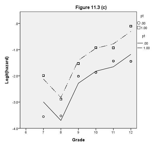
Figure 11.4, page 374
get file 'c:aldafirstsex_pp.sav'.
logistic regression var = event
 /method = enter d7 to d12 pt
 /origin
 /save pred (pred).

compute odds = pred/(1-pred).
compute logit = ln(odds).
execute.
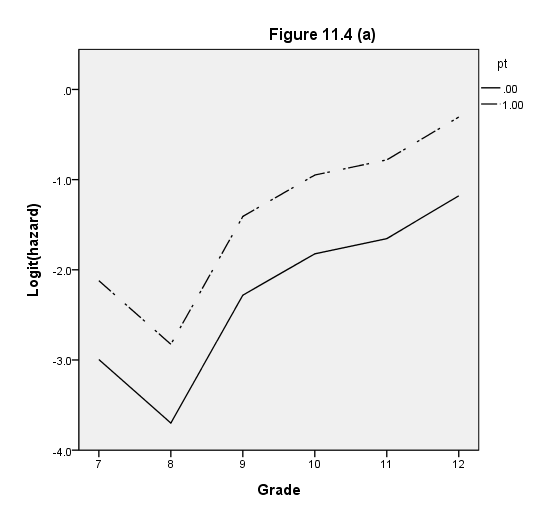
Top panel:
formats logit (f4.1) period (f2.0).
GGRAPH
  /GRAPHDATASET NAME="iGraphDataset" VARIABLES= logit period pt
  /GRAPHSPEC SOURCE=INLINE.
BEGIN GPL
SOURCE: s=userSource( id( "iGraphDataset" ) )
DATA: logit=col( source(s), name( "logit" ) )
DATA: period=col( source(s), name( "period" ) )
DATA: pt=col( source(s), name( "pt" ), unit.category()  )
GUIDE: text.title( label( "Figure 11.4 (a)" ) )
GUIDE: axis( dim( 1 ), label( "Grade" ) )
GUIDE: axis( dim( 2 ), label( "Logit(hazard)" ) )
GUIDE: legend( aesthetic( aesthetic.shape ), label( "pt" ) )
GUIDE: legend( aesthetic( aesthetic.shape.exterior ), label( "pt" ) )
SCALE: linear( dim( 1 ), min( 7 ), max( 12 ) )
SCALE: linear( dim( 2 ), min( -4 ), max( 0 ) )
SCALE: cat( aesthetic( aesthetic.shape ) )
ELEMENT: line( position( summary.mean( period * logit ) ), shape( pt )  )
END GPL.
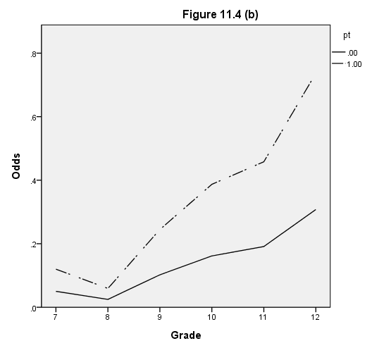
Middle panel:
formats odds (f4.1) period (f2.0).
GGRAPH
  /GRAPHDATASET NAME="iGraphDataset" VARIABLES= odds period pt
  /GRAPHSPEC SOURCE=INLINE.
BEGIN GPL
SOURCE: s=userSource( id( "iGraphDataset" ) )
DATA: odds=col( source(s), name( "odds" ) )
DATA: period=col( source(s), name( "period" ) )
DATA: pt=col( source(s), name( "pt" ), unit.category()  )
GUIDE: text.title( label( "Figure 11.4 (b)" ) )
GUIDE: axis( dim( 1 ), label( "Grade" ) )
GUIDE: axis( dim( 2 ), label( "Odds" ) )
GUIDE: legend( aesthetic( aesthetic.shape ), label( "pt" ) )
GUIDE: legend( aesthetic( aesthetic.shape.exterior ), label( "pt" ) )
SCALE: linear( dim( 1 ), min( 7 ), max( 12 ) )
SCALE: linear( dim( 2 ), min( 0 ), max( .8 ) )
SCALE: cat( aesthetic( aesthetic.shape ) )
ELEMENT: line( position( summary.mean( period * odds ) ), shape( pt )  )
END GPL.
Bottom panel:
formats pred (f4.1) period (f2.0).
GGRAPH
  /GRAPHDATASET NAME="iGraphDataset" VARIABLES= pred period pt
  /GRAPHSPEC SOURCE=INLINE.
BEGIN GPL
SOURCE: s=userSource( id( "iGraphDataset" ) )
DATA: pred=col( source(s), name( "pred" ) )
DATA: period=col( source(s), name( "period" ) )
DATA: pt=col( source(s), name( "pt" ), unit.category()  )
GUIDE: text.title( label( "Figure 11.4 (c)" ) )
GUIDE: axis( dim( 1 ), label( "Grade" ) )
GUIDE: axis( dim( 2 ), label( "Hazard" ) )
GUIDE: legend( aesthetic( aesthetic.shape ), label( "pt" ) )
GUIDE: legend( aesthetic( aesthetic.shape.exterior ), label( "pt" ) )
SCALE: linear( dim( 1 ), min( 7 ), max( 12 ) )
SCALE: linear( dim( 2 ), min( 0 ), max( .5 ) )
SCALE: cat( aesthetic( aesthetic.shape ) )
ELEMENT: line( position( summary.mean( period * pred ) ), shape( pt )  )
END GPL.
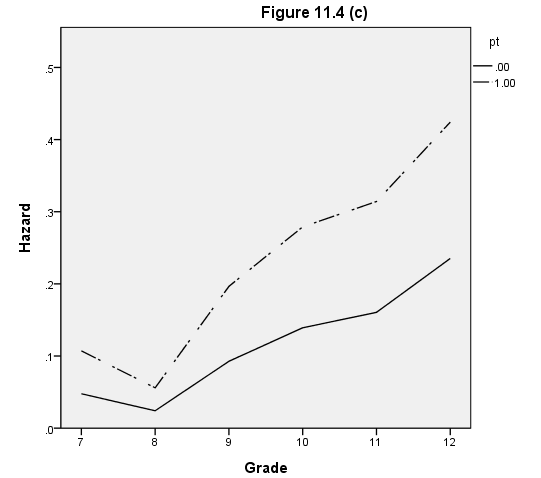
Table 11.3, page 386
Model A:
NOTE: The SPSS output has been abbreviated to save space.
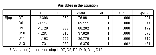
Because we entered all of the time dummies (d7 through d12), we need to omit the intercept. The /origin subcommand tells SPSS to omit the origin.
logistic regression var = event
 /method = enter d7 d8 d9 d10 d11 d12
 /origin.

Model B:
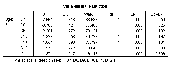
logistic regression var = event
 /method = enter d7 d8 d9 d10 d11 d12 pt
 /origin.


Model C:
logistic regression var = event
 /method = enter d7 d8 d9 d10 d11 d12 pas
 /origin.

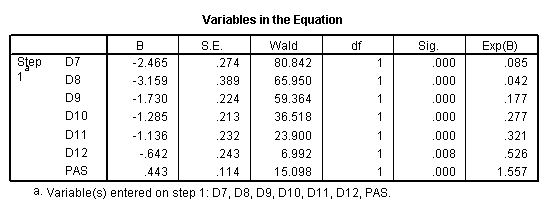
Model D:
logistic regression var = event
 /method = enter d7 d8 d9 d10 d11 d12 pt pas
 /origin.

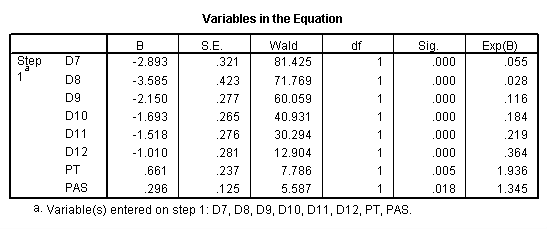
Table 11.4, page 388
This table is based on the output from Model A above. Because of the difficulty in outputting the parameter estimates into a data set, we simply created the data set by hand. Next, we use the compute command to get the fitted odds (fodds) and fitted hazard (fhazard), and then (after formatting the variables so that they look like those shown in the text), we use the list command to show the variables.
data list list
 /time parametr.
begin data.
7 -2.398
8 -3.117
9 -1.720
10 -1.287
11 -1.163
12 -.731
end data.

compute fodds = exp(parametr).
compute fhazard = 1/(1+exp(-parametr)).
execute.

formats time (F2.0) parametr fodds fhazard (F6.4).
list time parametr fodds fhazard.
TIME PARAMETR  FODDS FHAZARD

  7   -2.398   .0909   .0833
  8   -3.117   .0443   .0424
  9   -1.720   .1791   .1519
 10   -1.287   .2761   .2164
 11   -1.163   .3125   .2381
 12   -.7310   .4814   .3250


Number of cases read:  6    Number of cases listed:  6
Table 11.5, page 392
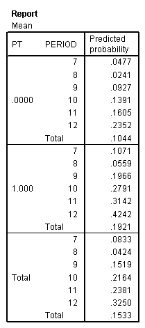
First, we run Model B from Table 11.3 and save the predicted values, which we call pred. The output from the logistic command gives the second and third columns of the table. The fourth column is the same as the second column, and the fifth column is obtained by adding the value of in the third column to that of the fourth. The means command gives the sixth and seventh columns of the table. The aggregate and casestovars commands are necessary to collapse the data and to reshape it. Compute commands are used to create the survivor functions, which are then formatted and listed. This provides the eighth and ninth columns of the table.
get file 'c:aldafirstsex_pp.sav'.

logistic regression var = event
 /method = enter d7 d8 d9 d10 d11 d12 pt
 /origin
 /save pred (pred).
means tables pred by pt by period
 /cells mean.
aggregate
/outfile='c:aldaaggr1.sav'
/break=period pt
/pred = mean(pred).

get file 'c:aldaaggr1.sav' .

sort cases by period.
casestovars
 /id = period
 /groupby = variable
 /vind.

* compute survival function.
compute s1 = 1-pred.1.
do if $casenum >=2.
compute t1= lag(s1).
compute s1 = t1* (1-pred.1).
end if.
execute.

compute s2 = 1-pred.2.
do if $casenum >=2.
compute t2= lag(s2).
compute s2 = t2* (1-pred.2).
end if.
execute.
save outfile 'c:aldaaggr2.sav'.
formats period (F2.0) s1 s2 (F6.4).
list period s1 s2.

PERIOD     S1     S2

   7    .9523  .8929
   8    .9293  .8430
   9    .8432  .6772
  10    .7259  .4882
  11    .6094  .3348
  12    .4660  .1928


Number of cases read:  6    Number of cases listed:  6
Figure 11.6, page 393
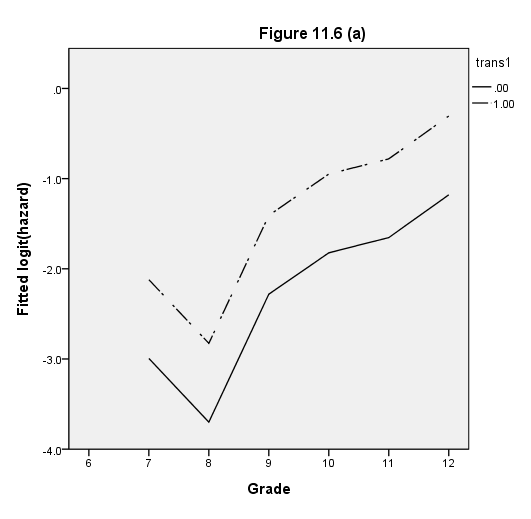
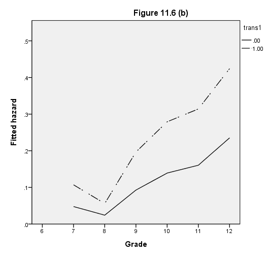
In order to make the graphs for this figure, we need to reshape the data file that we used above. We reshape the data file from wide to long using the varstocases command. Next, we use the compute command to calculate the odds and the logits that we need for the graphs. For each of the graphs, we double clicked on them and altered the appearance of the legend (to clarify it) and we altered the number of ticks on the x-axis. We changed the number of decimal places showing on both of the axes. These changes are only cosmetic and are not necessary to interpret the graph.
get file 'c:aldaaggr2.sav' .

varstocases
 /make trans1 from pt.1 pt.2
 /make trans2 from pred.1 pred.2
 /make trans3 from t1 t2
 /make trans4 from s1 s2
 /index = index1(trans1)
 /keep = period ind1 ind2.
Top panel:
compute odds = trans2/(1-trans2).
compute logit = ln(odds).
execute.

formats logit (f3.1) period (f2.0).
GGRAPH
  /GRAPHDATASET NAME="iGraphDataset" VARIABLES= logit period trans1
  /GRAPHSPEC SOURCE=INLINE.
BEGIN GPL
SOURCE: s=userSource( id( "iGraphDataset" ) )
DATA: logit=col( source(s), name( "logit" ) )
DATA: period=col( source(s), name( "period" ) )
DATA: trans1=col( source(s), name( "trans1" ), unit.category()  )
GUIDE: text.title( label( "Figure 11.6 (a)" ) )
GUIDE: axis( dim( 1 ), label( "Grade" ) )
GUIDE: axis( dim( 2 ), label( "Fitted logit(hazard)" ) )
GUIDE: legend( aesthetic( aesthetic.shape ), label( "trans1" ) )
GUIDE: legend( aesthetic( aesthetic.shape.exterior ), label( "trans1" ) )
SCALE: linear( dim( 1 ), min( 6 ), max( 12 ) )
SCALE: linear( dim( 2 ), min( -4 ), max( 0 ) )
SCALE: cat( aesthetic( aesthetic.color ) )
ELEMENT: line( position( summary.mean( period * logit ) ), shape( trans1 )  )
END GPL.
Middle panel:
formats trans2 (f3.1) period (f2.0).
GGRAPH
  /GRAPHDATASET NAME="iGraphDataset" VARIABLES= trans2 period trans1
  /GRAPHSPEC SOURCE=INLINE.
BEGIN GPL
SOURCE: s=userSource( id( "iGraphDataset" ) )
DATA: trans2=col( source(s), name( "trans2" ) )
DATA: period=col( source(s), name( "period" ) )
DATA: trans1=col( source(s), name( "trans1" ), unit.category()  )
GUIDE: text.title( label( "Figure 11.6 (b)" ) )
GUIDE: axis( dim( 1 ), label( "Grade" ) )
GUIDE: axis( dim( 2 ), label( "Fitted hazard" ) )
GUIDE: legend( aesthetic( aesthetic.shape ), label( "trans1" ) )
GUIDE: legend( aesthetic( aesthetic.shape.exterior ), label( "trans1" ) )
SCALE: linear( dim( 1 ), min( 6 ), max( 12 ) )
SCALE: linear( dim( 2 ), min( 0 ), max( 0.5 ) )
SCALE: cat( aesthetic( aesthetic.color ) )
ELEMENT: line( position( summary.mean( period * trans2 ) ), shape( trans1 )  )
END GPL.
Bottom panel:
formats trans4 (f3.1) period (f2.0).
GGRAPH
  /GRAPHDATASET NAME="iGraphDataset" VARIABLES= trans4 period trans1
  /GRAPHSPEC SOURCE=INLINE.
BEGIN GPL
SOURCE: s=userSource( id( "iGraphDataset" ) )
DATA: trans4=col( source(s), name( "trans4" ) )
DATA: period=col( source(s), name( "period" ) )
DATA: trans1=col( source(s), name( "trans1" ), unit.category()  )
GUIDE: text.title( label( "Figure 11.6 (c)" ) )
GUIDE: axis( dim( 1 ), label( "Grade" ) )
GUIDE: axis( dim( 2 ), label( "Fitted survival probability" ), delta(.5) )
GUIDE: legend( aesthetic( aesthetic.shape ), label( "trans1" ) )
GUIDE: legend( aesthetic( aesthetic.shape.exterior ), label( "trans1" ) )
GUIDE: form.line(position(*,.5), shape(shape.dash))
GUIDE: form.line(position(9.9), shape(shape.dash))
GUIDE: form.line(position(11.8), shape(shape.dash))
SCALE: linear( dim( 1 ), min( 6 ), max( 12 ) )
SCALE: linear( dim( 2 ), min( 0 ), max( 1 ) )
SCALE: cat( aesthetic( aesthetic.color ) )
ELEMENT: line( position( summary.mean( period * trans4 ) ), shape( trans1 )  )
END GPL.
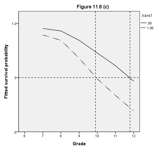
Figure 11.7, page 395
Top panel:
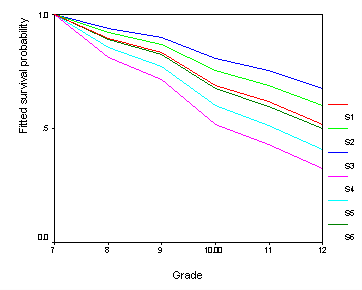
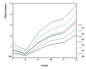
We begin by running Model D from Table 11.3 and save the predicted values, which we call pred. Next, we use the compute command to calculate the hazards for each of the six combinations of pt and pas. We use a multiple line graph to graph the six lines on the same graph.
* Model D from Table 11.3.

get file 'c:aldafirstsex_pp.sav'.

logistic regression var = event
 /method = enter d7 d8 d9 d10 d11 d12 pt pas
 /origin
 /save pred (pred).

compute h1= -2.893*d7-3.585*d8-2.15*d9-1.693*d10-1.518*d11-1.01*d12+0*.661+.296*1.
compute h2= -2.893*d7-3.585*d8-2.15*d9-1.693*d10-1.518*d11-1.01*d12+0*.661+.296*0.
compute h3= -2.893*d7-3.585*d8-2.15*d9-1.693*d10-1.518*d11-1.01*d12+0*.661+.296*(-1).
compute h4= -2.893*d7-3.585*d8-2.15*d9-1.693*d10-1.518*d11-1.01*d12+1*.661+.296*1.
compute h5= -2.893*d7-3.585*d8-2.15*d9-1.693*d10-1.518*d11-1.01*d12+1*.661+.296*0.
compute h6= -2.893*d7-3.585*d8-2.15*d9-1.693*d10-1.518*d11-1.01*d12+1*.661+.296*(-1).
execute.

compute a1 = 1/(1+(exp(-h1))).
compute a2 = 1/(1+(exp(-h2))).
compute a3 = 1/(1+(exp(-h3))).
compute a4 = 1/(1+(exp(-h4))).
compute a5 = 1/(1+(exp(-h5))).
compute a6 = 1/(1+(exp(-h6))).
execute.

graph
 /line(multiple) = mean(a1) mean(a2) mean(a3) mean(a4) mean(a5) mean(a6) by period.
Bottom panel:
In order to create the survival graph, we need to use the aggregate command to collapse the data. The /outfile subcommand saves the aggregated data file, and then we use the get file command to open the aggregated data file. We need to compute the survivor function for each of the six combinations of pt and pas. We could find no way to do this within a loop. Finally, we use the graph command to graph the six lines on a single graph.
aggregate
 /outfile = 'c:aldaaggr3.sav'
 /break = period
 /a1_1 = mean(a1)
 /a2_1 = mean(a2)
 /a3_1 = mean(a3)
 /a4_1 = mean(a4)
 /a5_1 =  mean(a5)
 /a6_1 = mean(a6).

get file 'c:aldaaggr3.sav'.

* pt = 0 and PAS = -1.
compute x1 = 1-a1_1.
do if $casenum >=2.
compute t1= lag(x1).
compute s1 = t1* (1-a1_1).
end if.
if $casenum = 1 s1 = 1.
execute.

* pt = 0 and PAS = 0.
compute x2 = 1-a2_1.
do if $casenum >=2.
compute t2= lag(x2).
compute s2 = t2* (1-a2_1).
end if.
if $casenum = 1 s2 = 1.
execute.

* pt = 0 and PAS = 1.
compute x3 = 1-a3_1.
do if $casenum >=2.
compute t3= lag(x3).
compute s3 = t3* (1-a3_1).
end if.
if $casenum = 1 s3 = 1.
execute.

* pt = 1 and PAS = -1.
compute x4 = 1-a4_1.
do if $casenum >=2.
compute t4= lag(x4).
compute s4 = t4* (1-a4_1).
end if.
if $casenum = 1 s4 = 1.
execute.

* pt = 1 and PAS = 0.
compute x5 = 1-a5_1.
do if $casenum >=2.
compute t5= lag(x5).
compute s5 = t5* (1-a5_1).
end if.
if $casenum = 1 s5 = 1.
execute.

* pt = 1 and PAS = 1.
compute x6 = 1-a6_1.
do if $casenum >=2.
compute t6= lag(x6).
compute s6 = t6* (1-a6_1).
end if.
if $casenum = 1 s6 = 1.
execute.

graph
 /line(multiple) = mean(s1) mean(s2) mean(s3) mean(s4) mean(s5) mean(s6) by period.
