Table 12.2, page 413
Selected smooth polynomial representations for the main effect of time in a discrete-time hazard model. First we get the data and then we have to create the higher order terms for time. Finally we run the logistic regression entering the higher order time variables in separate blocks so that SPSS will compare the deviance scores between the models.
get file= 'c:\temp\tenure_pp.sav'.

*Creating the variables used in table 12_2.

compute one = 1.
compute time = period.
compute time2 = period**2.
compute time3 = period**3.
compute time4 = period**4.
compute time5 = period**5.
execute.

logistic regression var=event
  /method=enter one
  /method=enter time
  /method=enter time2
  /method=enter time3
  /method=enter time4
  /method=enter time5
  /origin.
Constant Model:

Linear Model:


Quadratic Model:


Cubic Model:


Fourth Order Model:


Fifth Order Model:


The General Model:

logistic regression var=event
 /method=enter d1 to d9
 /origin.

--------------------------------------------------------------------------
Figure 12.1, page 414
Computing the variables need for Figure 12.1
*saving the predicted values--constant model.
logistic regression var=event
 /method=enter one
 /origin
 /save pred (haz0).

*computing the fitted logit(hazard) functions for constant model.
compute x0 = -ln( (1-haz0) / haz0 ).
execute.

*saving the predicted values--linear model.
logistic regression var=event
 /method=enter one time
 /origin
 /save pred (haz1).

*computing the fitted logit(hazard) functions for linear model.
compute x1 = -ln( (1-haz1) / haz1 ).
execute.

*saving the predicted values--quadratic model.
logistic regression var=event
 /method=enter one time time2
 /origin
 /save pred (haz2).

*computing the fitted logit(hazard) functions for quadratic model.
compute x2 = -ln( (1-haz2) / haz2 ).
execute.

*saving the predicted values--cubic model.
logistic regression var=event
 /method=enter one time time2 time3
 /origin
 /save pred (haz3).

*computing the fitted logit(hazard) functions for cubic model.
compute x3 = -ln( (1-haz3) / haz3 ).
execute.

*saving the predicted values--general model.
logistic regression var=event
 /method=enter d1 to d9
 /origin
 /save pred (hazg).

*computing the fitted logit(hazard) functions for general model.
compute xg = -ln( (1-hazg) / hazg ).
execute.

sort cases by period (A).
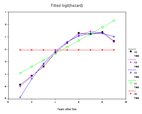
Figure 12.1–top panel
graph
 /scatterplot(overlay) = time time time time time  WITH x0 x1 x2 x3 xg (PAIR).

 Note: The graphs have been manipulated manually after running the graph commands.
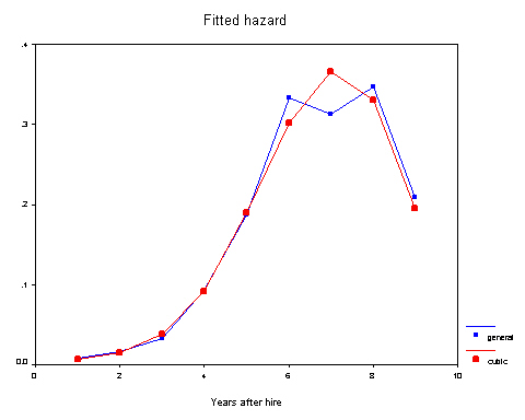
Figure 12.1–lower right panel
graph
 /scatterplot(overlay) = time time with haz3 hazg (PAIR).
Figure 12.1–lower left panel
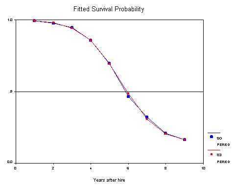
*Compute the survival functions for cubic and general models.
aggregate
 /outfile='c:\temp\aggr.sav'
 /break=period
 /hazg = mean(hazg)
 /haz3 = mean(haz3).

get file='c:\temp\aggr.sav'.

compute s3 = 1-haz3.
compute sg = 1-hazg.
do if $casenum >=2.
compute t3= lag(s3).
compute tg= lag(sg).
compute s3 = t3*(1-haz3).
compute sg = tg*(1-hazg).
end if.
execute.

graph
 /scatterplot(overlay) = period period with s3 sg (PAIR).
--------------------------------------------------------------------------
Figure 12.6, page 445
Top two panels skipped for now.
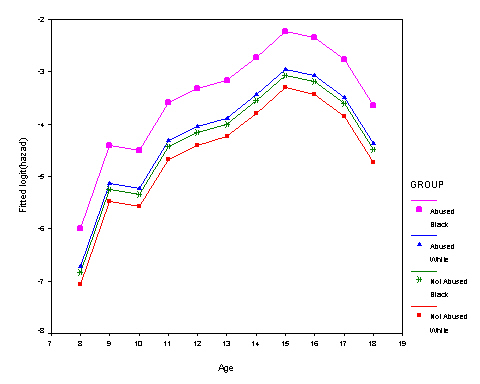
Figure 12.6–bottom panel
get file= 'c:\temp\firstarrest_pp.sav'.

logistic regression var=event
 /method=enter abused black ablack d8 to d18
 /origin
 /save pred (haz).

*computing the logit(hazard) and group variable.
compute logit = -ln( (1-haz) / haz ).
if abused=0 & black=0 group=0.
if abused=0 & black=1 group=1.
if abused=1 & black=0 group=2.
if abused=1 & black=1 group=3.
exe.

sort cases by period.

graph
 /scatterplot period with logit by group.

 Note: The graph has been manipulated manually after running the graph command.
--------------------------------------------------------------------------
Table 12.4, page 449
Table 12.4–Model A
get file= 'c:\temp\depression_pp.sav'.

logistic regression var=event
 /method=enter one age_18 age_18sq age_18cu pd female nsibs
 /origin.

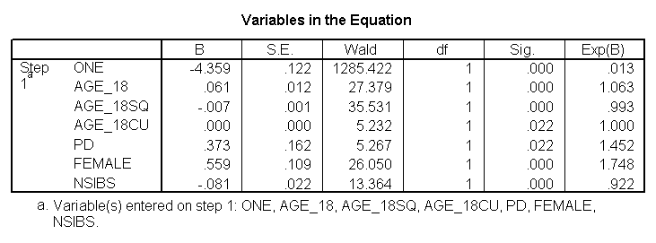
Table 12.4–Model B
logistic regression var=event
 /method=enter one age_18 age_18sq age_18cu pd female
  sibs12 sibs34 sibs56 sibs78 sibs9plu
 /origin.

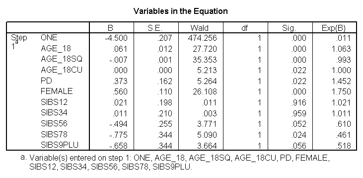
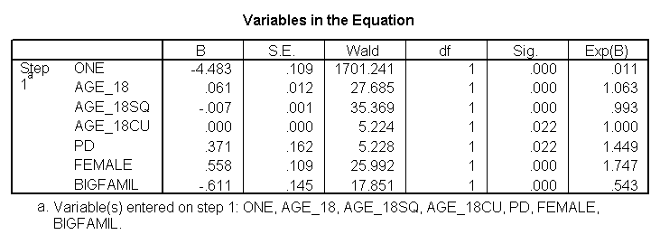
Table 12.4–Model C
logistic regression var=event
 /method=enter one age_18 age_18sq age_18cu pd female bigfamil
 /origin.

--------------------------------------------------------------------------
Table 12.5, page 459
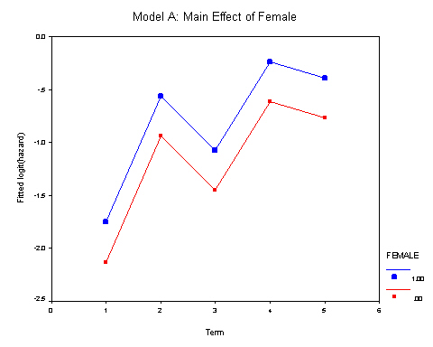
Table 12.5–Model A The /save subcommand is used to save the hazard function for model A which will be used in Figure 12.8
get file= 'c:\temp\mathdropout_pp.sav'.
logistic regression var=event
 /method=enter hs11 hs12 coll1 coll2 coll3 female
 /origin
 /save pred (haz_a).


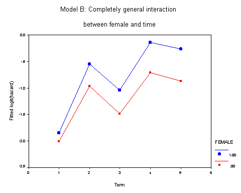
Table 12.5–Model B The /save subcommand is used to save the hazard function for model B which will be used in Figure 12.8
logistic regression var=event
 /method=enter hs11 hs12 coll1 coll2 coll3 fhs11 fhs12 fcoll1 fcoll2 fcoll3
 /origin
 /save pred (haz_b).

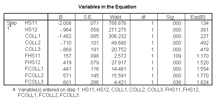
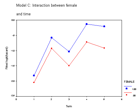
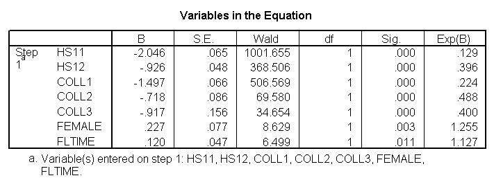
Table 12.5–Model C The /save subcommand is used to save the hazard function for model C which will be used in Figure 12.8
logistic regression var=event
 /method=enter hs11 hs12 coll1 coll2 coll3 female fltime
 /origin
 /save pred (haz_c).

————————————————————————–
Figure 12.8, page 458
Computing the variables need for Figure 12.8. Note you need to run the commands for Table 12.5 before running the following set of commands.
compute logit_a = -ln( (1-haz_a) / haz_a ).
compute logit_b = -ln( (1-haz_b) / haz_b ).
compute logit_c = -ln( (1-haz_c) / haz_c ).
execute.

sort cases by period.
Figure 12.8–top right panel
graph
 /scatterplot = period with logit_a by female.

 Note: The graphs have been manipulated manually after the graph commands.
Figure 12.8–bottom left panel
graph
 /scatterplot = period with logit_b by female.
Figure 12.8–bottom right panel
graph
 /scatterplot = period with logit_c by female.

