Table 13.2, page 477
NOTE: The code below gives columns 1 through 4 and 8 through 9 of the table. Also note that the labels used in the text are very different from those used in the SPSS output. The table below matches the labels.
Column label in text Column label in SPSS output n at risk Number entrng this intrvl n events Number of termnl events n censored Number wdrawn during intrvl Actuarial estimates (survival) Cumul propn surv at end Actuarial estimates (hazard) Hazard rate
get file 'c:aldahonking.sav'.

survival table = seconds
 /interval = thru 8 by 1
 /status=censor(0)
 /print=table.
This subfile contains:      57 observations

 Life Table
   Survival Variable  SECONDS

        Number  Number  Number  Number                  Cumul
Intrvl  Entrng  Wdrawn  Exposd    of    Propn   Propn   Propn   Proba-
Start    this   During    to    Termnl  Termi-  Sur-    Surv    bility  Hazard
Time    Intrvl  Intrvl   Risk   Events  nating  viving  at End  Densty   Rate
------  ------  ------  ------  ------  ------  ------  ------  ------  ------
    .0    57.0      .0    57.0      .0   .0000  1.0000  1.0000   .0000   .0000
   1.0    57.0     1.0    56.5     5.0   .0885   .9115   .9115   .0885   .0926
   2.0    51.0     3.0    49.5    14.0   .2828   .7172   .6537   .2578   .3294
   3.0    34.0     2.0    33.0     9.0   .2727   .7273   .4754   .1783   .3158
   4.0    23.0     4.0    21.0     6.0   .2857   .7143   .3396   .1358   .3333
   5.0    13.0     2.0    12.0     2.0   .1667   .8333   .2830   .0566   .1818
   6.0     9.0     2.0     8.0     2.0   .2500   .7500   .2122   .0707   .2857
   7.0     5.0      .0     5.0     1.0   .2000   .8000   .1698   .0424   .2222
   8.0+    4.0     1.0     3.5     3.0   .8571   .1429   .0243     **      **

 **     These calculations for the last interval are meaningless.

 The median survival time for these data is   3.86

         SE of   SE of
 Intrvl  Cumul   Proba-  SE of
 Start   Sur-    bility  Hazard
 Time    viving  Densty   Rate
-------  ------  ------  ------
     .0   .0000   .0000   .0000
    1.0   .0378   .0378   .0414
    2.0   .0643   .0593   .0868
    3.0   .0690   .0536   .1039
    4.0   .0680   .0508   .1342
    5.0   .0674   .0383   .1280
    6.0   .0666   .0465   .2000
    7.0   .0654   .0402   .2208
    8.0+  .0331     **      **
Table 13.3, page 484
NOTE: The code below gives columns 4, 8 and 11 of the table. Also note that SPSS "number remaining" column is the "n at risk" column in the text, except the values are shifted by one line. We use the /save survival subcommand to save the survival estimates to our data set for use in the next figure.
km seconds
 /status=censor(0)
 /print table
 /save survival.
 Survival Analysis for SECONDS

  Time       Status       Cumulative     Standard     Cumulative      Number
                           Survival       Error         Events       Remaining

    1.41          .00        .9825          .0174              1            56
    1.41         1.00                                          1            55
    1.51          .00        .9646          .0246              2            54
    1.67          .00        .9467          .0299              3            53
    1.68          .00        .9289          .0343              4            52
    1.86          .00        .9110          .0380              5            51
    2.12          .00        .8931          .0412              6            50
    2.19          .00        .8753          .0441              7            49
    2.36         1.00                                          7            48
    2.48          .00        .8570          .0468              8            47
    2.50          .00        .8388          .0492              9            46
    2.53          .00        .8206          .0514             10            45
    2.54          .00        .8023          .0534             11            44
    2.56          .00        .7841          .0552             12            43
    2.62          .00        .7659          .0569             13            42
    2.68          .00        .7476          .0584             14            41
    2.76         1.00                                         14            40
    2.78         1.00                                         14            39
    2.83          .00        .7285          .0599             15            38
    2.88          .00        .7093          .0614             16            37
    2.89          .00        .6901          .0626             17            36
    2.92          .00        .6710          .0637             18            35
    2.98          .00        .6518          .0647             19            34
    3.05         1.00                                         19            33
    3.14          .00        .6320          .0657             20            32
    3.17          .00        .6123          .0666             21            31
    3.21          .00        .5925          .0673             22            30
    3.22          .00        .5728          .0679             23            29
    3.24          .00        .5530          .0684             24            28
    3.46         1.00                                         24            27
    3.56          .00        .5325          .0688             25            26
    3.57          .00        .5121          .0692             26            25
    3.58          .00        .4916          .0694             27            24
    3.78          .00        .4711          .0694             28            23
    4.01         1.00                                         28            22
    4.10          .00        .4497          .0695             29            21
    4.18          .00        .4283          .0694             30            20
    4.30         1.00                                         30            19
    4.44          .00        .4057          .0693             31            18
    4.51          .00        .3832          .0690             32            17
    4.52          .00        .3606          .0686             33            16
    4.63         1.00                                         33            15
    4.71         1.00                                         33            14
    4.96          .00        .3349          .0683             34            13
    5.12         1.00                                         34            12
    5.39          .00        .3070          .0681             35            11
    5.73          .00        .2791          .0674             36            10
    5.88         1.00                                         36             9
    6.03          .00        .2481          .0666             37             8
    6.21         1.00                                         37             7
    6.30          .00        .2126          .0659             38             6
    6.60         1.00                                         38             5
    7.20          .00        .1701          .0650             39             4
    9.59          .00        .1276          .0611             40             3
   12.29          .00        .0851          .0535             41             2
   13.18          .00        .0425          .0403             42             1
   17.15         1.00                                         42             0

 Number of Cases:  57        Censored:   15     ( 26.32%)   Events: 42
Figure 13.2, page 485
Top panel:
Note that we modified the graph produced by the code below by double clicking on the graph to open the Chart Editor and then double clicking on the elements that we wanted to change, such as the labeling of the axes. We used the "Interpolation" button at the top of the Chart Editor to delete the symbols and use a step function to connect the points.
sort cases by sur_1.
graph scatterplot(bivar)= seconds with sur_1.
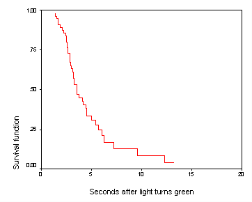
Bottom panel:
We do not know how to overlay the different survival functions onto a single graph in SPSS.
Figure 13.4, page 493
This has been skipped for now.
Figure 13.5, page 496
This has been skipped for now.
Figure 13.6, page 499
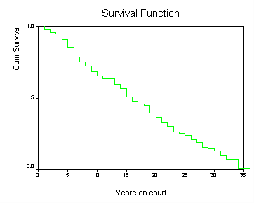
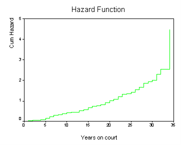
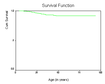
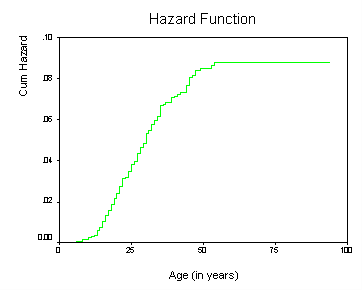
NOTE: We do not know how to do smoothed graphs in SPSS, so the third graph in each column has been omitted.
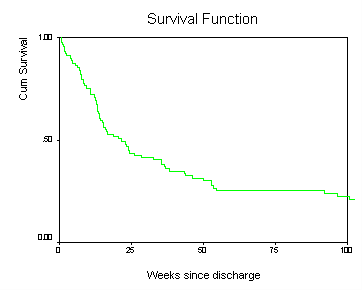
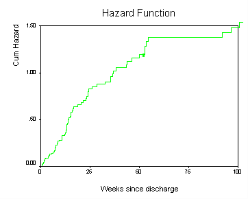
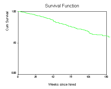
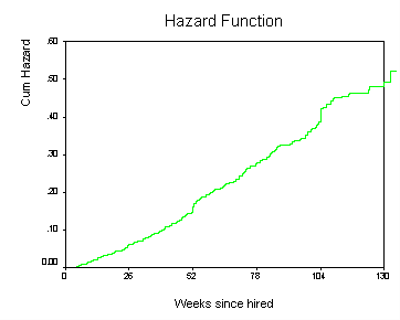
get file 'c:aldaalcohol_relapse.sav'. km weeks /status=censor(0) /print none /plot survival hazard.get file 'c:aldajudges.sav'. km tenure /status=leave(1) /print none /plot survival hazard.get file 'c:aldafirstdepression.sav'. km age /status=censor(0) /print none /plot survival hazard.get file 'c:aldahealthworkers.sav'. km weeks /status=censor(0) /print none /plot survival hazard.
