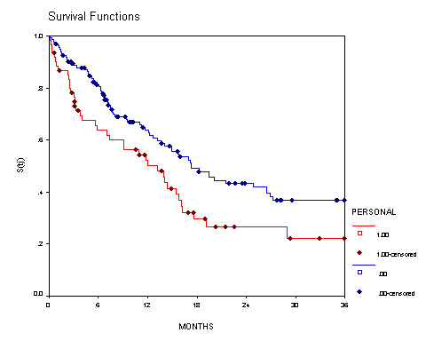
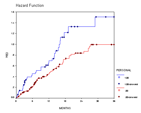
Applied Longitudinal Data Analysis: Modeling Change and Event Occurrence by Judith D. Singer and John B. Willett Chapter 14: Fitting Cox regression models

Figure 14.1, page 505

The top panel represents the estimated survivor function for the recidivism data stratified by the predictor personal; the bottom panel represents the cumulative hazard function also stratified by personal. Note that the graphs have been manipulated manually after running the syntax.

get file='c:aldarearrest.sav'.

KM months BY personal  
  /status=censor(0)
  /print none
  /plot survival hazard.

Table 14.1, page 525

Note that in SPSS using the Efron method to break ties is not an option, instead all Cox regression will use the Breslow method for breaking ties which is the default in SPSS.

Model A: Including only the predictor personal.

coxreg months
 /status=censor(0)
 /method=enter personal.

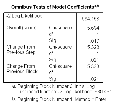
We can also get the likelihood-ratio test shown at the lower part of Table 14.1 by using stepwise approach. Here is the code for it.

coxreg months
 /status=censor(0)
 /method=fstep(lr) personal.

Model B: Including only the predictor property.

coxreg months
 /status=censor(0)
 /method=enter property.

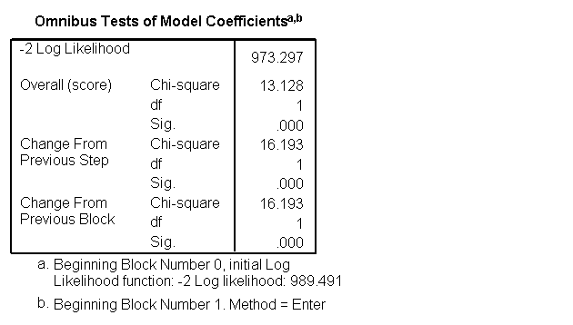
Again, we can get likelihood-ratio test by using stepwise approach with L-R tests as shown below.

coxreg months /status=censor(0) /method=fstep(lr) property.

Model C: Including only the predictor age (centered).

coxreg months
 /status=censor(0)
 /method=enter cage.

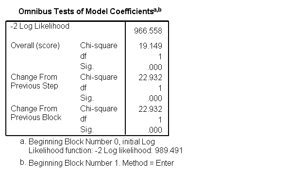
Again, we can get likelihood-ratio test by using stepwise approach with L-R tests as shown below.

coxreg months
 /status=censor(0)
 /method=fstep(lr) cage.

Model D: Including all three predictors personal, property and age.

coxreg months
 /status=censor(0)
 /method=enter personal property cage.

Again, we can get likelihood-ratio test by using stepwise approach with L-R tests as shown below.

coxreg months /status=censor(0) /method=fstep(lr) personal property cage.

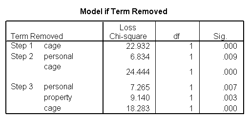
Table 14.2, page 533

Risk scores estimated from model D in Table 14.1 for select individuals.

coxreg months
 /status=censor(0)
 /method=enter personal property cage.

*computing the risk score.
compute risk = exp(.569*personal + .935*property - .067*cage).
exe.

use all.
compute filter_$=(id=22|id=8|id=187|id=26|id=5|id=130|id=106|id=33).
filter by filter_$.
exe.

list id personal property cage risk months censor.

filter off.
use all.
exe.

      id personal property     cage     risk   months   censor

    5.00     1.00     1.00    -7.16     7.27      .30      .00
    8.00     1.00     1.00    22.45     1.00      .62     1.00
   22.00      .00      .00      .26      .98     1.71     1.00
   26.00      .00     1.00    -7.30     4.15     2.37      .00
   33.00     1.00      .00    27.06      .29     2.79     1.00
  106.00      .00      .00    16.20      .34    11.70      .00
  130.00      .00     1.00    22.39      .57    15.97     1.00
  187.00     1.00      .00    -7.20     2.86    36.00     1.00

Figure 14.4 on page 538

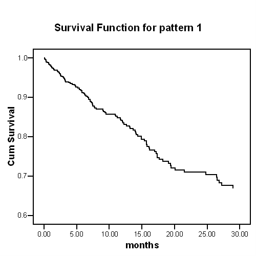
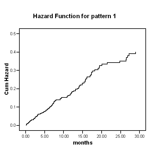
Left panels: Baseline survivor function and cumulative hazard function for model D in Table 14.1. The baseline is for all covariates set equal to zero. The bottom plot is a smoothed hazard function and we omit it here.

coxreg months  
 /status=censor(0)
 /method=enter personal property cage  
 /plot survival hazard
 /pattern personal(0) property(0) cage(0).

Right panels: Using model D in Table 14.1 but with all the predictors centered and the baseline is for all the centered covariates set equal to zero (which since the predictors are centered is equal to all the variables set equal to their means). The bottom plot is a smoothed hazard function plot and we omit it here.

compute cper = personal- mean(personal).
compute cprop = property - mean(property).
exe. 

*necessary?.
coxreg months  
 /status=censor(0)
 /method=enter cper cprop cage  
 /plot survival hazard.

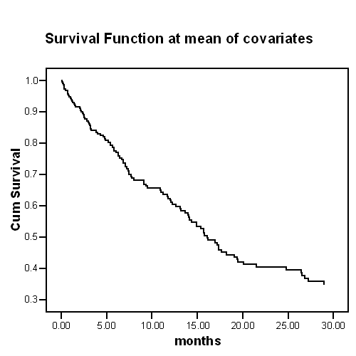
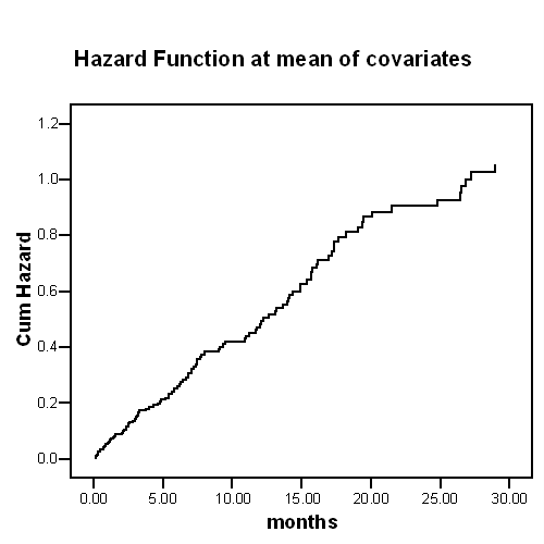
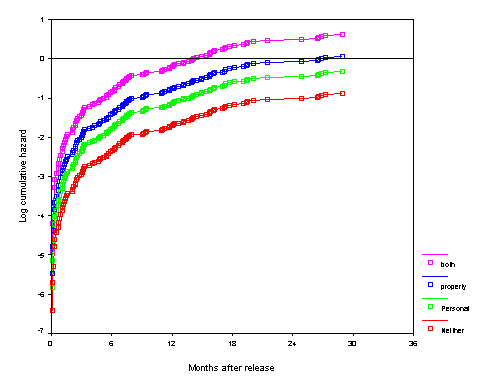
Figure 14.5, page 541

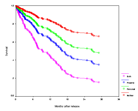
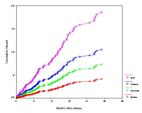
Survival, cumulative hazard and log-cumulative hazard functions for model D in table 14.1 for age set at its mean and varying the values of the other predictors personal and property.

First we save the cumulative hazard function and the xbeta score which will be used to calculate the baseline score when all the variables are set to zero. XBETA in SPSS is the linear combination of mean corrected covariates times regression coefficients from the model. Therefore, the relationship between the cumulative hazard function and the xbeta score is

H(t)/exp(xbeta) = H₀(t)*exp(the linear combination of mean values of covariates times regression coefficients)
= H₀(t)*exp(0.5691*.314 + 0.9358*.814 + (-.067)*0)
= H₀(t)*2.5611.

Here .314 is the mean for variable personal and .814 is the mean for variable property and 0 is the mean for variable cage since it is centered. Therefore, the baseline hazard function is H₀(t) = H(t)/(exp(xbeta)*2.5611).

coxreg months  
 /status=censor(0)
 /method=enter personal property cage  
 /save= hazard (haz) xbeta (xbeta1)
 /print= baseline.

compute haz1 = haz/( exp( xbeta1) ).
compute haz0 = haz1 / 2.5611.
compute hazper = haz0*exp(0.5691).
compute hazprop = haz0*exp(0.9358).
compute hazboth = haz0*exp(1.5049).
compute surv0 = exp(-haz0).
compute survper = exp(-hazper).
compute survprop = exp(-hazprop).
compute survboth = exp(-hazboth).
compute logh0 = ln(haz0).
compute loghper = ln(hazper).
compute loghprop = ln(hazprop).
compute loghboth = ln(hazboth).
exe.

use all.
compute filter_$= censor=0.
filter by filter_$.
exe.

graph 
/scatterplot(overlay) = months months months months with 
                     haz0 hazper hazprop hazboth (pair).

graph 
/scatterplot(overlay) = months months months months with 
                     surv0 survper survprop survboth (pair).

graph 
/scatterplot(overlay) = months months months months with 
                     logh0 loghper loghprop loghboth (pair).

filter off.
use all.
exe.