This page was done using SPSS 12.
Table 15.1, page 548. Notice that the results don’t match with the results in the table completely. This is due to the fact that SPSS does not use the Efron method to deal with tied observations.
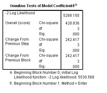
Model A: Predictors include birthyr and the time-invariant predictors earlymj and earlyod.
get file='c:aldafirstcocaine.sav'.

coxreg cokeage
 /status=censor(0)
 /method=enter birthyr earlymj earlyod.

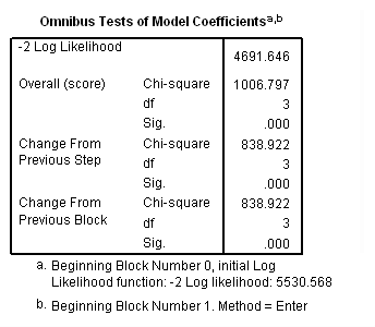
Model B: Predictors include birthyr and the time-varying predictors usedmj and usedod.
time program.
compute T_usedmj = mjyes = 1 and mjage < T_.
compute T_usedod = odyes = 1 and odage < T_.
coxreg cokeage
 /status=censor(0)
 /method=enter birthyr T_usedmj T_usedod.

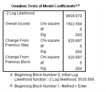
Model C: Includes predictor birthyr and the time-varying predictors usedmj, soldmj, usedod and moreod.
time program.
compute T_usedmj = mjyes = 1 and mjage < T_.
compute T_soldmj = sellmjye=1 and sellmjag < T_.
compute T_usedod = odyes = 1 and odage < T_.
compute T_moreod = sdyes = 1 and sdage < T_.
coxreg cokeage
 /status=censor(0)
 /method=enter birthyr T_usedmj T_soldmj T_usedod T_moreod.

Model D: Includes predictor birthyr, the time-invariant predictors earlymj and earlyod as well as the time-varying predictors usedmj, soldmj, usedod and moreod.
time program.
compute T_usedmj = mjyes = 1 and mjage < T_.
compute T_soldmj = sellmjye=1 and sellmjag < T_.
compute T_usedod = odyes = 1 and odage < T_.
compute T_moreod = sdyes = 1 and sdage < T_.
coxreg cokeage
 /status=censor(0)
 /method=enter birthyr earlymj T_usedmj T_soldmj earlyod T_usedod T_moreod.
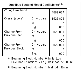
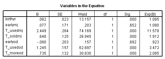
Table 15.2 on page 555. Comparing alternative imputation strategies for time-varying predictors.
Model A: Predictors include needle and basemood.
get file='c:aldarelapse_days2.sav'.

coxreg days
 /status=censor(0)
 /method=enter nasal basemood.


Model B: Predictors include needle and weekmood.
time program.
compute week = trunc(T_/7) +1.
if (week=1)  T_weekmd = weekmood.
if (week=2)  T_weekmd = weekmoo1.
if (week=3)  T_weekmd = weekmoo2.
if (week=4)  T_weekmd = weekmoo3.
if (week=5)  T_weekmd = weekmoo4.
if (week=6)  T_weekmd = weekmoo5.
if (week=7)  T_weekmd = weekmoo6.
if (week=8)  T_weekmd = weekmoo7.
if (week=9)  T_weekmd = weekmoo8.
if (week=10) T_weekmd = weekmoo9.
if (week=11) T_weekmd = weekmo10.
if (week=12) T_weekmd = weekmo11.
coxreg days
 /status=censor(0)
 /method=enter nasal T_weekmd.


Model C– skipped for now.
Figure 15.2 on page 559 using data set firstcocaine.sav.
get file='c:aldafirstcocaine.sav'.
COXREG cokeage
/STATUS=censor(0)
/STRATA=rural
/PLOT LML
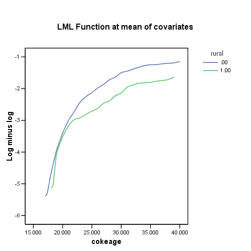
Table 15.3, page 560
Column I: The unstratified model (Model C).
get file='c:aldafirstcocaine.sav'.

time program.
compute T_usedmj = mjyes = 1 and mjage < T_.
compute T_soldmj = sellmjye=1 and sellmjag < T_.
compute T_usedod = odyes = 1 and odage < T_.
compute T_moreod = sdyes = 1 and sdage < T_.
coxreg cokeage
 /status=censor(0)
 /method=enter birthyr T_usedmj T_soldmj T_usedod T_moreod.


Column II: Stratified by RURAL.
time program.
compute T_usedmj = mjyes = 1 and mjage < T_.
compute T_soldmj = sellmjye=1 and sellmjag < T_.
compute T_usedod = odyes = 1 and odage < T_.
compute T_moreod = sdyes = 1 and sdage < T_.
coxreg cokeage
 /status=censor(0)
 /method=enter birthyr T_usedmj T_soldmj T_usedod T_moreod
 /stratum=rural.


Column III and IV: Fitting the model separately for each level of rural.
sort cases by rural.
split file by rural.

time program.
compute T_usedmj = mjyes = 1 and mjage < T_.
compute T_soldmj = sellmjye=1 and sellmjag < T_.
compute T_usedod = odyes = 1 and odage < T_.
compute T_moreod = sdyes = 1 and sdage < T_.
coxreg cokeage
 /status=censor(0)
 /method=enter birthyr T_usedmj T_soldmj T_usedod T_moreod.
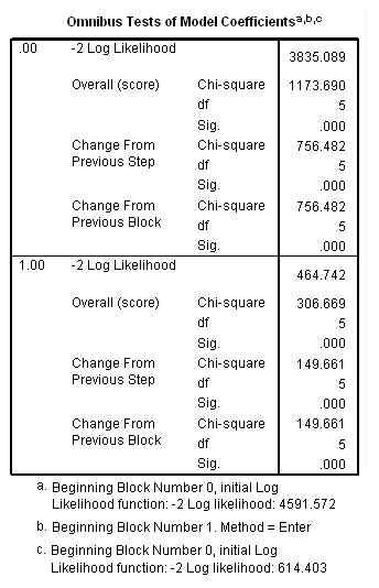
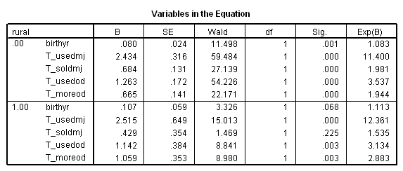
Table 15.4, page 566
Fitting non-proportional hazards Cox regression models.
Model A: Predictors include the main effect of treat.
get file='c:aldalengthofstay.sav'.

coxreg days
 /status=censor(0)
 /method=enter treat.
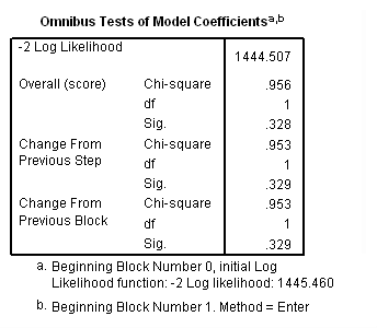

Model B: The effects of treat vary linearly over time.
time program.
compute T_treat = treat*(T_ -1).
coxreg days
 /status= censor(0)
 /method=enter treat T_treat.


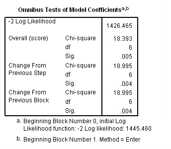
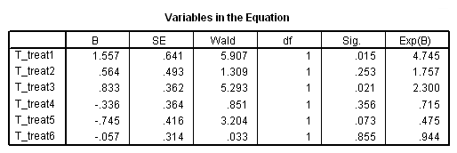
Model C: The effects of treat differ week by week.
time program.
compute T_treat1=0.
if (T_ le 7) T_treat1=treat.
compute T_treat2=0.
if (T_ > 7 & T_ le 14) T_treat2=treat.
compute T_treat3=0.
if (T_> 14 & T_ le 21) T_treat3=treat.
compute T_treat4=0.
if (T_ > 21 & T_ le 28) T_treat4=treat.
compute T_treat5=0.
if (T_ > 28 & T_ le 35) T_treat5=treat.
compute T_treat6=0.
if (T_ > 35) T_treat6=treat.
coxreg days
 /status=censor(0)
 /method=enter T_treat1 to T_treat6.
Model D: The effects of treat varies linearly with the logarithm of base 10 of time.
time program.
compute T_lgtrt = treat*lg10(T_)/lg10(2).
coxreg days
 /status=censor(0)
 /method=enter treat T_lgtrt.


Figure 15.3 on page 567, top panel.
COXREG
  days
  /STATUS=censor(0)
  /STRATA=treat
  /PLOT  LML .
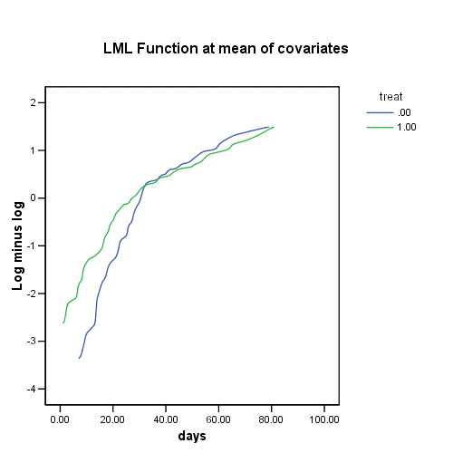
Figure 15.3, lower panel.
COXREG
  days  /STATUS=censor(0)  /STRATA=treat
  /SAVE=LML.

SAVE OUTFILE='D:aldaspssfig15_3.sav'
 /COMPRESSED.

FILTER OFF.
USE ALL.
SELECT IF(treat = 0).
EXECUTE .
rename variable (LML_1 = lml_t0).
SAVE OUTFILE='D:aldaspsstreat_0.sav'
  /DROP=id censor /COMPRESSED.

GET FILE='D:aldaatsdataspsslengthofstay_fig15_3.sav'.
FILTER OFF.
USE ALL.
SELECT IF(treat = 1).
EXECUTE .
rename variable (LML_1 = lml_t1).
SAVE OUTFILE='D:aldaspsstreat_1.sav'
  /DROP=id censor /COMPRESSED.

MATCH FILES /FILE=*
 /RENAME (censor id = d0 d1)
 /FILE='D:aldaatsdataspsstreat_0.sav'
 /RENAME (treat = d2)
 /BY days
 /DROP= d0 d1 d2.
EXECUTE.
COMPUTE diff = lml_t1 - lml_t0 .
EXECUTE .
GRAPH
  /SCATTERPLOT(BIVAR)=days WITH diff.
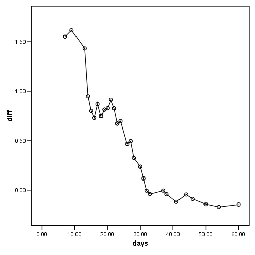
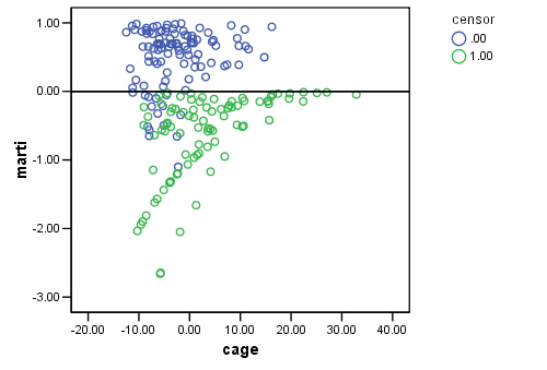
Figure 15.4 on page 573, top panel. By the definition given in the book, we can manually compute the martingale residuals as shown below and then plot them again variable cage.
GET
  FILE='D:aldaspssrearrest.sav'.
COXREG months
   /STATUS=censor(0)
   /SAVE=HAZARD (HAZ_1).
COMPUTE marti = 1- censor - HAZ_1.
EXECUTE .
GRAPH
  /SCATTERPLOT(BIVAR)=cage WITH marti BY censor
  /MISSING=LISTWISE .
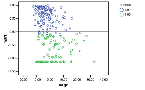
Figure 15.4, bottom panel.
COXREG
  months  /STATUS=censor(0)
  /METHOD = ENTER cage personal property
   /SAVE=HAZARD (HAZ_2).
COMPUTE marti = 1- censor - HAZ_2.
EXECUTE .
GRAPH
  /SCATTERPLOT(BIVAR)=cage WITH marti BY censor
  /MISSING=LISTWISE .
Figure 15.5 on page 576 using the rearrest.sav data.
GET FILE='D:aldaspssrearrest.sav'.
COXREG months  /STATUS=censor(0)
  /METHOD = ENTER cage personal property
  /SAVE=HAZARD(haz)  XBETA(xb).
COMPUTE marti = 1- censor - haz.
EXECUTE.

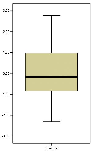
if (marti >=0) deviance = sqrt(-2*(marti + (1-censor)*ln(1-censor - marti))).
if (marti <0 ) deviance = - sqrt(-2*(marti + (1-censor)*ln(1-censor - marti))).
EXAMINE VARIABLES=deviance
  /PLOT BOXPLOT STEMLEAF.
deviance Stem-and-Leaf Plot

 Frequency    Stem &  Leaf

     4.00       -2 .  0033
    14.00       -1 .  55556666788999
    21.00       -1 .  000000000011222333334
    35.00       -0 .  55555555566666666677777788888999999
    29.00       -0 .  00000111222222222333444444444
    18.00        0 .  000011123344444444
    31.00        0 .  5555666667788888888899999999999
    19.00        1 .  0000001111113334444
    16.00        1 .  5555555666788899
     6.00        2 .  001244
     1.00        2 .  7

 Stem width:      1.00
 Each leaf:       1 case(s)
GRAPH
  /SCATTERPLOT(BIVAR)= xb WITH deviance BY censor
  /MISSING=LISTWISE .
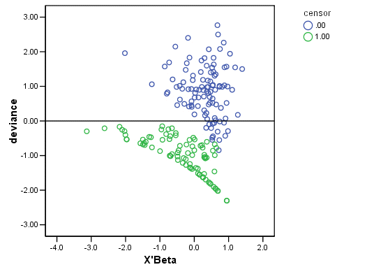
Figure 15.6 on page 580.
COXREG
  months
  /METHOD = ENTER cage personal property
 /STATUS=censor(0)
  /SAVE=presid.

RANK VARIABLES=months.
GRAPH
  /SCATTERPLOT(BIVAR)=Rmonths WITH PR2_2
  /MISSING=LISTWISE .
GRAPH
  /SCATTERPLOT(BIVAR)=Rmonths WITH PR3_2
  /MISSING=LISTWISE .
GRAPH
  /SCATTERPLOT(BIVAR)=Rmonths WITH PR1_2
  /MISSING=LISTWISE .
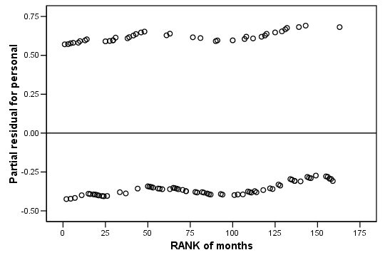
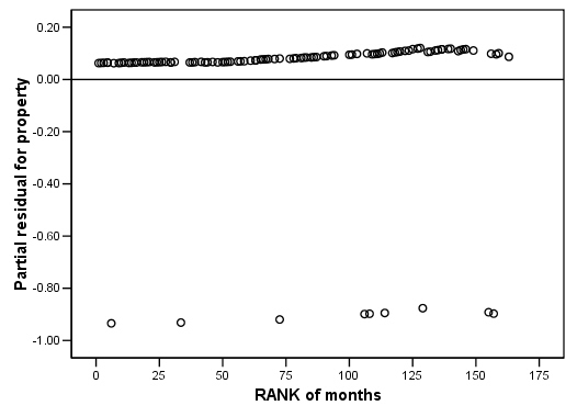
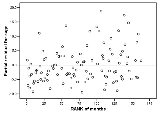
Figure 15.7 on page 583 using score residuals. SPSS does not save score residual variables, instead it has DFBETA variables which is a weighted transform of the score residual variables. So we will present the plots of DFBETA versus rank of months here.
COXREG
  months
  /METHOD = ENTER cage personal property
 /STATUS=censor(0)
  /SAVE=dfbeta (dfbeta).
GRAPH
  /SCATTERPLOT(BIVAR)=Rmonths WITH dfbeta2 BY censor.
GRAPH
  /SCATTERPLOT(BIVAR)=Rmonths WITH dfbeta3 BY censor.
GRAPH
 /SCATTERPLOT(BIVAR)=Rmonths WITH dfbeta1 BY censor.
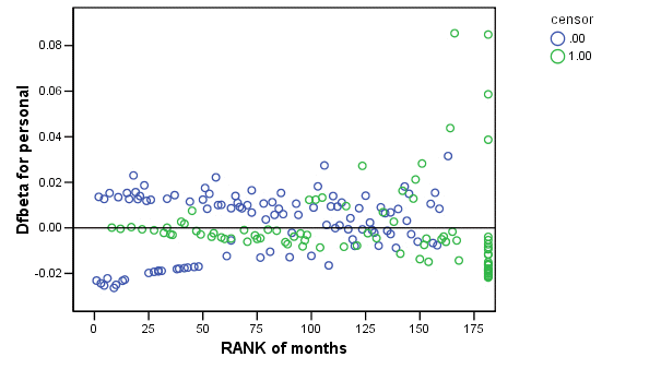
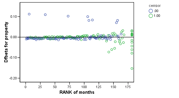
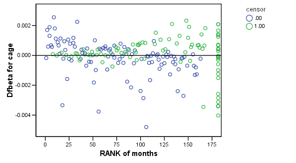
Table 15.6, page 587
Illustrates the structure of the Supreme Court data set by displaying the data for three individual judges.
get file='c:aldajudges.sav'.

compute left=0.
if (retire=1) left=1.
if (dead=1) left=2.
value labels left 0 "censored" 1 "retired" 2 "dead".
compute yearleft = year + age.
if (left=0) yearleft=$sysmis.
exe.

use all.
compute filter_$ =(id=2|id=13|id=107).
filter by filter_$.
exe.

list id year yearleft left tenure dead retire leave.

filter off.
use all.
exe.

     ID YEAR YEARLEFT     LEFT   TENURE     DEAD RETIRE    LEAVE

    2.00 1789  1846.00     1.00     6.00      .00   1.0      1.00
   13.00 1801  1846.00     2.00    34.00     1.00   .00      1.00
  107.00 1991      .        .00     8.00      .00   .00       .00
Figure 14.8 on page 589. skipped for now since SPSS 12 does not do overlay plots with connecting data points option.
Table 15.7, page 592
Competing-risk survival analysis.
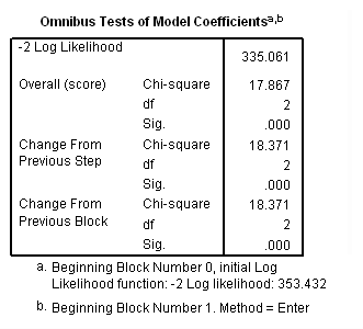
Model A: Fitting the model for the event of death only.
coxreg tenure
 /status= left(2)
 /method=enter age year.

Model B: Fitting the model for the event of retirement only.
coxreg tenure
 /status= left(1)
 /method=enter age year.


Model C: Fitting the model for the events of death and retirement.
coxreg tenure
 /status= left(1 2)
 /method=enter age year.


Table 15.8, page 601
Model A has been skipped because it is not possible to include late entry into the risk set in the coxreg command in SPSS.
Model B: Fitting the model only to those physicians hired during the measurement window.
get file='c:aldadoctors.sav'.

use all.
compute filter_$ = entry=0.
filter by filter_$.
exe.

time program.
compute T_yrage = T_*age.
coxreg exit
 /status=censor(0)
 /method=enter parttime age T_yrage.

filter off.
use all.
exe.
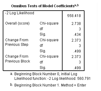

Model C: Ignoring the effects of late entrants. Beware that this is an incorrect model shown for pedagogical purposes only.
time program.
compute T_yrage = T_*age.
coxreg exit
 /status=censor(0)
 /method=enter parttime age T_yrage.


Table 15.9, page 604
Empirically comparing alternative metrics for clocking time in Cox regression analysis
Model A: Clocks time using session number.
get file='c:aldamonkeys.sav'.

coxreg sessions
 /status= censor(0)
 /method=enter female bodywt initial.


Model B: Clocks time using age but not accounting for late entry into the risk set.
coxreg end_age
 /status= censor(0)
 /method=enter female bodywt initial.


Model C has been skipped since it is currently not possible to include late entry in the coxreg command in SPSS.

