Please note that the "early_int" data file (which is used in Chapter 3) is not included among the data files. This was done at the request of the researchers who contributed this data file to ensure the privacy of the participants in the study. Although the web page shows how to obtain the results with this data file, we regret that visitors do not have access to this file to be able to replicate the results for themselves.
Table 3.1, page 48
compute filter = 0.
if any(id,68,70,71,72,902,904,906,908) filter = 1.
filter by filter.
list id age cog program.
execute.
use all.
      ID      AGE      COG  PROGRAM

     902     1.00   119.00      .00
     902     1.50    93.00      .00
     902     2.00    99.00      .00
     904     1.00   112.00      .00
     904     1.50    98.00      .00
     904     2.00    79.00      .00
     906     1.00    89.00      .00
     906     1.50    66.00      .00
     906     2.00    81.00      .00
     908     1.00   117.00      .00
     908     1.50    90.00      .00
     908     2.00    76.00      .00
      68     1.00   103.00     1.00
      68     1.50   119.00     1.00
      68     2.00    96.00     1.00
      70     1.00   106.00     1.00
      70     1.50   107.00     1.00
      70     2.00    96.00     1.00
      71     1.00   112.00     1.00
      71     1.50    86.00     1.00
      71     2.00    73.00     1.00
      72     1.00   100.00     1.00
      72     1.50    93.00     1.00
      72     2.00    87.00     1.00


Number of cases read:  24    Number of cases listed:  24
Figure 3.1, page 50
formats age (f4.1) cog (f4.0) id (f2.0)..
GGRAPH
  /GRAPHDATASET NAME="GraphDataset" VARIABLES= cog age id
  /GRAPHSPEC SOURCE=INLINE
INLINETEMPLATE=["<setWrapPanels/>"].
BEGIN GPL
SOURCE: s=userSource( id( "GraphDataset" ) )
DATA: cog=col( source(s), name( "cog" ) )
DATA: age=col( source(s), name( "age" ) )
DATA: id=col( source(s), name( "id" ), unit.category() )
GUIDE: text.title( label( "Figure 3.1" ) )
GUIDE: axis( dim( 1 ), label( "age" ), delta(.5) )
GUIDE: axis( dim( 2 ), label( "cog" ), delta(25) )
GUIDE: axis( dim( 3 ), label( "id" ), opposite() )
SCALE: linear( dim( 1 ), min(1), max(2) )
SCALE: linear( dim( 2 ), min(50), max(150) )
ELEMENT: point( position( ( age * cog * id ) ) )
ELEMENT: line( position(smooth.linear( age * cog * id) ))
END GPL.
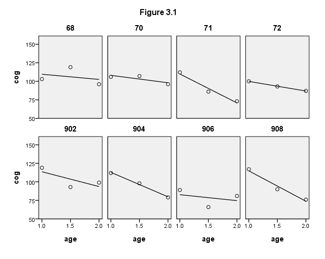
Figure 3.3, page 57.
formats age (f4.1) cog (f4.0).
GGRAPH
  /GRAPHDATASET NAME="GraphDataset" VARIABLES= cog age id
  /GRAPHSPEC SOURCE=INLINE .
BEGIN GPL
SOURCE: s=userSource( id( "GraphDataset" ) )
DATA: cog=col( source(s), name( "cog" ) )
DATA: age=col( source(s), name( "age" ) )
DATA: id=col( source(s), name( "id" ), unit.category() )
GUIDE: text.title( label( "Figure 3.3" ) )
GUIDE: axis( dim( 1 ), label( "age" ), delta(.5) )
GUIDE: axis( dim( 2 ), label( "cog" ), delta(25) )
GUIDE: legend(aesthetic(aesthetic.shape), null())
SCALE: linear( dim( 1 ), min(1), max(2) )
SCALE: linear( dim( 2 ), min(50), max(150) )
ELEMENT: line( position(smooth.linear( age * cog ) ), shape(id))
END GPL.
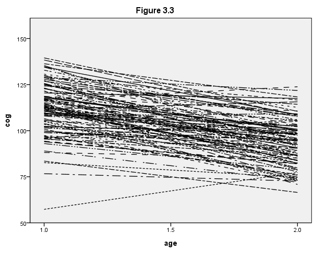
We can produce the stem-and-leaf plots for the fitted initial status and the fitted rate of change as follows.
sort cases by id.
split file by id.
REGRESSION
/DEPENDENT cog
/METHOD=ENTER time
/OUTFILE=COVB('D:aldafig3_3.sav').

GET FILE='D:aldafig3_3.sav'.
FILTER OFF.
USE ALL.
SELECT IF(rowtype_ = "EST").
EXECUTE .

examine variables=const_ time/plot=stemleaf.
Constant
Constant Stem-and-Leaf Plot
Frequency Stem & Leaf
     1.00 Extremes    (=<57)
     1.00        7 .  6
     2.00        8 .  23
     2.00        8 .  89
     3.00        9 .  344
    12.00        9 .  555666779999
     8.00       10 .  01222233
    14.00       10 .  55556688899999
    19.00       11 .  0000111222223333444
    13.00       11 .  5666677778888
     8.00       12 .  01122344
    11.00       12 .  55556778899
     5.00       13 .  00244
     4.00       13 .  5689
 Stem width:     10.00
 Each leaf:       1 case(s)
TIME
TIME Stem-and-Leaf Plot
Frequency Stem & Leaf
     6.00       -4 .  111344
     3.00       -3 .  789
    12.00       -3 .  000001223344
    13.00       -2 .  5566777789999
    14.00       -2 .  00001111222344
    14.00       -1 .  55666677888899
    13.00       -1 .  0001122233334
    14.00       -0 .  56777788889999
     7.00       -0 .  2334444
     3.00        0 .  134
     2.00        0 .  79
     1.00        1 .  0
     1.00 Extremes    (>=20)
 Stem width:     10.00
 Each leaf:       1 case(s)
Figure 3.4, page 59
use all.
value labels program 0 "program = 0" 1 "program = 1".
GGRAPH
  /GRAPHDATASET NAME="GraphDataset" VARIABLES= cog age id program
  /GRAPHSPEC SOURCE=INLINE .
BEGIN GPL
SOURCE: s=userSource( id( "GraphDataset" ) )
DATA: cog=col( source(s), name( "cog" ) )
DATA: age=col( source(s), name( "age" ) )
DATA: id=col( source(s), name( "id" ), unit.category() )
DATA: program=col( source(s), name( "program" ), unit.category() )
GUIDE: text.title( label( "Figure 3.4" ) )
GUIDE: axis( dim( 1 ), label( "age" ), delta(.5) )
GUIDE: axis( dim( 2 ), label( "cog" ), delta(25) )
GUIDE: axis( dim( 3 ), label( " " ), opposite() )
GUIDE: legend(aesthetic(aesthetic.shape), null())
SCALE: linear( dim( 1 ), min( 1 ), max( 2 ) )
SCALE: linear( dim( 2 ), min( 50 ), max( 150 ) )
ELEMENT: line( position(smooth.linear( age * cog * program) ), shape(id))
ELEMENT: line( position(smooth.linear( age * cog * program)), color(color.red) )
END GPL.
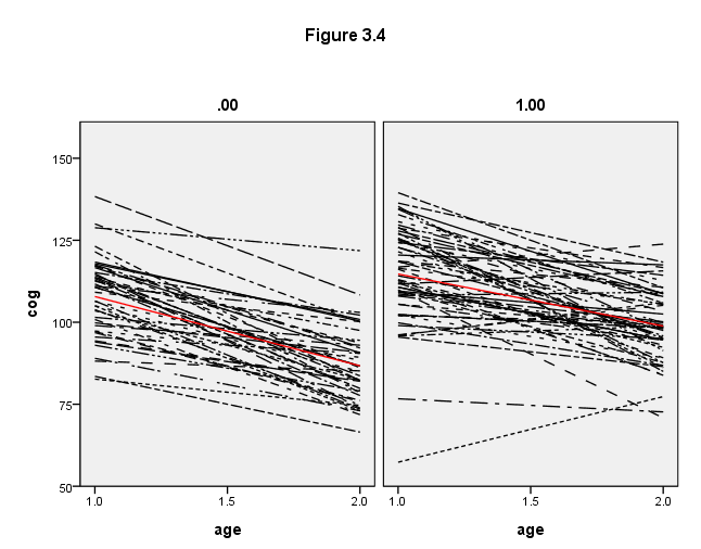
Table 3.3, page 69. Notice the warning message from SPSS output. The variance-covariance matrix is problematic. We haven’t been able to coerce SPSS to converge to the right variance-covariance matrix on this model.
compute time1 = age - 1.
execute.

mixed cog with time1 program
 /print = solution
 /method = ml
 /fixed = time1 program time1*program
 /random intercept time1 | subject(id) covtype(un).
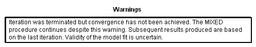
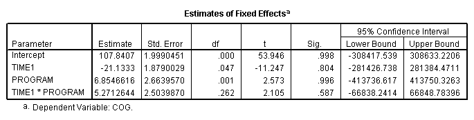
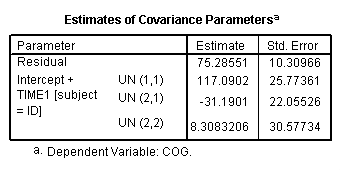
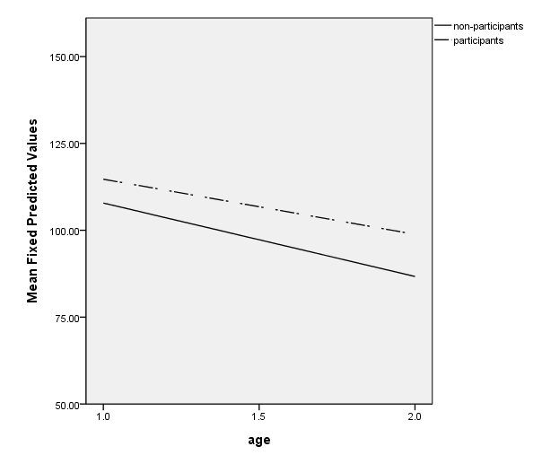
Figure 3.5, page 71
mixed cog with time1 program
 /method = ml
 /fixed = time1 program time1*program
 /random intercept time1 | subject(id) covtype(un)
/save = fixpred(pred).
value labels program 0 "non-participants" 1 "participants".

GGRAPH
  /GRAPHDATASET NAME="graphdataset" VARIABLES=age MEAN(pred)[name="MEAN_pred"] program
  /GRAPHSPEC SOURCE=INLINE.
BEGIN GPL
SOURCE: s=userSource(id("graphdataset"))
DATA: age=col(source(s), name("age"))
DATA: MEAN_pred=col(source(s), name("MEAN_pred"))
DATA: program=col(source(s), name("program"), unit.category())
GUIDE: axis(dim(1), label("age"), delta(.5))
GUIDE: axis(dim(2), label("Mean Fixed Predicted Values"), delta(25))
GUIDE: legend(aesthetic(aesthetic.color.interior), label("program"))
SCALE: linear(dim(1), min(1), max(2))
SCALE: linear(dim(2), min(50), max(150))
ELEMENT: line(position(age*MEAN_pred), shape(program))
END GPL.