page 269 The regressions at the bottom of the page.
GET FILE='D:davis.sav'.
For the uncorrected data:
compute measf = measwt*female.
execute.

regression
 /dep=reptwt
 /method=enter measwt female measf.
| Model | Variables Entered | Variables Removed | Method |
|---|---|---|---|
| 1 | MEASF, Measured Weight, Gender, 0=male, 1=female(a) | . | Enter |
| a All requested variables entered. | |||
| b Dependent Variable: Reported Weight | |||
| Model | R | R Square | Adjusted R Square | Std. Error of the Estimate |
|---|---|---|---|---|
| 1 | .942(a) | .887 | .886 | 4.661 |
| a Predictors: (Constant), MEASF, Measured Weight, Gender, 0=male, 1=female | ||||
| Model | Sum of Squares | df | Mean Square | F | Sig. | |
|---|---|---|---|---|---|---|
| 1 | Regression | 30654.729 | 3 | 10218.243 | 470.408 | .000(a) |
| Residual | 3888.254 | 179 | 21.722 | |
|
|
| Total | 34542.984 | 182 | |
|
|
|
| a Predictors: (Constant), MEASF, Measured Weight, Gender, 0=male, 1=female | ||||||
| b Dependent Variable: Reported Weight | ||||||
| |
Unstandardized Coefficients | Standardized Coefficients | t | Sig. | ||
|---|---|---|---|---|---|---|
| Model | B | Std. Error | Beta | |||
| 1 | (Constant) | 1.359 | 3.277 | |
.415 | .679 |
| Measured Weight | .990 | .043 | 1.099 | 23.236 | .000 | |
| Gender, 0=male, 1=female | 39.964 | 3.929 | 1.447 | 10.171 | .000 | |
| MEASF | -.725 | .056 | -1.611 | -12.957 | .000 | |
| a Dependent Variable: Reported Weight | ||||||
For the corrected data:
compute nmwt = measwt.
if subject=12 nmwt=57.
if subject=12 measht=166.
compute measwtf = nmwt*female.
execute.

regression
 /dep=reptwt
 /method=enter nmwt female measwtf.
| Model | Variables Entered | Variables Removed | Method |
|---|---|---|---|
| 1 | MEASWTF, NMWT, Gender, 0=male, 1=female(a) | . | Enter |
| a All requested variables entered. | |||
| b Dependent Variable: Reported Weight | |||
| Model | R | R Square | Adjusted R Square | Std. Error of the Estimate |
|---|---|---|---|---|
| 1 | .987(a) | .974 | .973 | 2.243 |
| a Predictors: (Constant), MEASWTF, NMWT, Gender, 0=male, 1=female | ||||
| Model | Sum of Squares | df | Mean Square | F | Sig. | |
|---|---|---|---|---|---|---|
| 1 | Regression | 33642.345 | 3 | 11214.115 | 2228.780 | .000(a) |
| Residual | 900.639 | 179 | 5.032 | |
|
|
| Total | 34542.984 | 182 | |
|
|
|
| a Predictors: (Constant), MEASWTF, NMWT, Gender, 0=male, 1=female | ||||||
| b Dependent Variable: Reported Weight | ||||||
| |
Unstandardized Coefficients | Standardized Coefficients | t | Sig. | ||
|---|---|---|---|---|---|---|
| Model | B | Std. Error | Beta | |||
| 1 | (Constant) | 1.359 | 1.577 | |
.861 | .390 |
| NMWT | .990 | .021 | .962 | 48.279 | .000 | |
| Gender, 0=male, 1=female | 1.983 | 2.450 | .072 | .809 | .420 | |
| MEASWTF | -5.668E-02 | .038 | -.119 | -1.474 | .142 | |
| a Dependent Variable: Reported Weight | ||||||
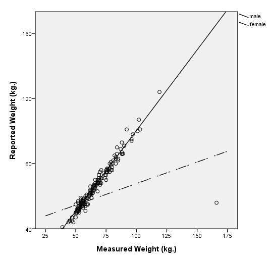
page 270 Figure 11.2 Davis's data on reported and measured weight for women (F) and men (M), showing the least-squares linear regression line for each group (the broken line for men, the solid line for women). The outlying observation has a substantial effect on the fitted line for women.
USE ALL.
COMPUTE filter_$=(female=1).
VARIABLE LABEL filter_$ 'female=1 (FILTER)'.
VALUE LABELS filter_$  0 'Not Selected' 1 'Selected'.
FORMAT filter_$ (f1.0).
FILTER BY filter_$.
EXECUTE.

formats reptwt measwt (f4.0).

GGRAPH
  /GRAPHDATASET NAME="GraphDataset" VARIABLES= reptwt measwt female
  /GRAPHSPEC SOURCE=INLINE.
BEGIN GPL
SOURCE: s=userSource( id( "GraphDataset" ) )
DATA: reptwt=col( source(s), name( "reptwt" ) )
DATA: measwt=col( source(s), name( "measwt" ) )
DATA: female = col(source(s), name("female"), unit.category())
GUIDE: axis( dim( 1 ), label( "Measured Weight (kg.)" ), start(0.0), delta(25) )
GUIDE: axis( dim( 2 ), label( "Reported Weight (kg.)" ), start(0.0), delta(40) )
SCALE: linear( dim( 1 ), min(25), max(175) )
SCALE: linear( dim( 2 ), min(40), max(160) )
ELEMENT: point( position(measwt * reptwt))
ELEMENT: line(position(smooth.linear(measwt * reptwt)), shape(female))
END GPL.

page 271 The largest hat value (middle of the page).
NOTE: Various statistics, including DFBETAs, studentized residuals and covariance ratios, are discussed in this section. Those statistics have been calculated and displayed by the regression command below.
GET FILE='D:davis.sav'.

compute rptfem = reptwt*female.
execute.

regression
 /dep=measwt
 /method=enter reptwt female rptfem
 /save lev sres dfbeta covratio.
| Model | Variables Entered | Variables Removed | Method |
|---|---|---|---|
| 1 | RPTFEM, Reported Weight, Gender, 0=male, 1=female(a) | . | Enter |
| a All requested variables entered. | |||
| b Dependent Variable: Measured Weight | |||
| Model | R | R Square | Adjusted R Square | Std. Error of the Estimate |
|---|---|---|---|---|
| 1 | .837(a) | .700 | .695 | 8.449 |
| a Predictors: (Constant), RPTFEM, Reported Weight, Gender, 0=male, 1=female | ||||
| b Dependent Variable: Measured Weight | ||||
| Model | Sum of Squares | df | Mean Square | F | Sig. | |
|---|---|---|---|---|---|---|
| 1 | Regression | 29786.378 | 3 | 9928.793 | 139.071 | .000(a) |
| Residual | 12779.436 | 179 | 71.393 | |
|
|
| Total | 42565.814 | 182 | |
|
|
|
| a Predictors: (Constant), RPTFEM, Reported Weight, Gender, 0=male, 1=female | ||||||
| b Dependent Variable: Measured Weight | ||||||
| |
Unstandardized Coefficients | Standardized Coefficients | t | Sig. | ||
|---|---|---|---|---|---|---|
| Model | B | Std. Error | Beta | |||
| 1 | (Constant) | 1.794 | 5.924 | |
.303 | .762 |
| Reported Weight | .969 | .076 | .873 | 12.681 | .000 | |
| Gender, 0=male, 1=female | 2.074 | 9.297 | .068 | .223 | .824 | |
| RPTFEM | -9.525E-03 | .147 | -.018 | -.065 | .948 | |
| a Dependent Variable: Measured Weight | ||||||
| Case Number | Std. Residual | Measured Weight |
|---|---|---|
| 12 | 12.830 | 166 |
| a Dependent Variable: Measured Weight | ||
| |
Minimum | Maximum | Mean | Std. Deviation | N |
|---|---|---|---|---|---|
| Predicted Value | 43.20 | 121.94 | 66.22 | 12.793 | 183 |
| Std. Predicted Value | -1.799 | 4.355 | .000 | 1.000 | 183 |
| Standard Error of Predicted Value | .841 | 3.743 | 1.183 | .402 | 183 |
| Adjusted Predicted Value | 43.49 | 122.66 | 66.24 | 12.811 | 183 |
| Residual | -7.66 | 108.41 | .00 | 8.380 | 183 |
| Std. Residual | -.906 | 12.830 | .000 | .992 | 183 |
| Stud. Residual | -.935 | 12.895 | -.001 | .997 | 183 |
| Deleted Residual | -8.15 | 109.50 | -.01 | 8.475 | 183 |
| Stud. Deleted Residual | -.935 | 48.221 | .192 | 3.580 | 183 |
| Mahal. Distance | .810 | 34.720 | 2.984 | 3.619 | 183 |
| Cook's Distance | .000 | .421 | .003 | .031 | 183 |
| Centered Leverage Value | .004 | .191 | .016 | .020 | 183 |
| a Dependent Variable: Measured Weight | |||||
NOTE: SPSS values for the leverage do not exactly match those obtained by Fox.
compute measf = measwt*female.
execute.

regression
 /dep=reptwt
 /method=enter measwt female measf
 /save lev.
| Model | Variables Entered | Variables Removed | Method |
|---|---|---|---|
| 1 | MEASF, Measured Weight, Gender, 0=male, 1=female(a) | . | Enter |
| a All requested variables entered. | |||
| b Dependent Variable: Reported Weight | |||
| Model | R | R Square | Adjusted R Square | Std. Error of the Estimate |
|---|---|---|---|---|
| 1 | .942(a) | .887 | .886 | 4.661 |
| a Predictors: (Constant), MEASF, Measured Weight, Gender, 0=male, 1=female | ||||
| b Dependent Variable: Reported Weight | ||||
| Model | Sum of Squares | df | Mean Square | F | Sig. | |
|---|---|---|---|---|---|---|
| 1 | Regression | 30654.729 | 3 | 10218.243 | 470.408 | .000(a) |
| Residual | 3888.254 | 179 | 21.722 | |
|
|
| Total | 34542.984 | 182 | |
|
|
|
| a Predictors: (Constant), MEASF, Measured Weight, Gender, 0=male, 1=female | ||||||
| b Dependent Variable: Reported Weight | ||||||
| |
Unstandardized Coefficients | Standardized Coefficients | t | Sig. | ||
|---|---|---|---|---|---|---|
| Model | B | Std. Error | Beta | |||
| 1 | (Constant) | 1.359 | 3.277 | |
.415 | .679 |
| Measured Weight | .990 | .043 | 1.099 | 23.236 | .000 | |
| Gender, 0=male, 1=female | 39.964 | 3.929 | 1.447 | 10.171 | .000 | |
| MEASF | -.725 | .056 | -1.611 | -12.957 | .000 | |
| a Dependent Variable: Reported Weight | ||||||
| Case Number | Std. Residual | Reported Weight |
|---|---|---|
| 12 | -6.270 | 56 |
| 115 | 3.342 | 77 |
| a Dependent Variable: Reported Weight | ||
| |
Minimum | Maximum | Mean | Std. Deviation | N |
|---|---|---|---|---|---|
| Predicted Value | 51.64 | 119.15 | 65.62 | 12.978 | 183 |
| Std. Predicted Value | -1.078 | 4.124 | .000 | 1.000 | 183 |
| Standard Error of Predicted Value | .464 | 3.939 | .618 | .306 | 183 |
| Adjusted Predicted Value | 51.99 | 158.24 | 66.01 | 14.583 | 183 |
| Residual | -29.22 | 15.58 | .00 | 4.622 | 183 |
| Std. Residual | -6.270 | 3.342 | .000 | .992 | 183 |
| Stud. Residual | -11.728 | 3.392 | -.029 | 1.241 | 183 |
| Deleted Residual | -102.24 | 16.04 | -.39 | 8.643 | 183 |
| Stud. Deleted Residual | -24.304 | 3.497 | -.096 | 2.008 | 183 |
| Mahal. Distance | .808 | 128.987 | 2.984 | 9.774 | 183 |
| Cook's Distance | .000 | 85.927 | .474 | 6.352 | 183 |
| Centered Leverage Value | .004 | .709 | .016 | .054 | 183 |
| a Dependent Variable: Reported Weight | |||||
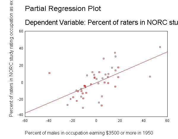
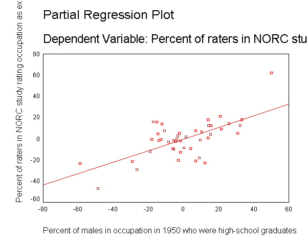
page 284 Figure 11.5 Partial-regression plots for Duncan's regression of occupational prestige on the income (a) and educational levels (b) of 45 U.S. occupations. in 1950. Three potentially influential observations (ministers, railroad conductors, and railroad engineers) are identified on the plots. The partial-regression plot for the intercept A is not shown.
NOTE: In order to get the regression line on the plot, you need to use the code below, double-click on the resulting graph, select chart from the menu at the top, select options, click on fit line total, select fit options, select regression, click on continue and OK. We do not know how to add the regression line using code.
GET FILE='D:duncan.sav'.

regression
 /dep=prestige
 /method=enter income educ
 /partialplot all
 /sav sresid lev cook.
| Model | Variables Entered | Variables Removed | Method |
|---|---|---|---|
| 1 | Percent of males in occupation in 1950 who were high-school graduates, Percent of males in occupation earning $3500 or more in 1950(a) | . | Enter |
| a All requested variables entered. | |||
| b Dependent Variable: Percent of raters in NORC study rating occupation as excellent or good in presti | |||
| Model | R | R Square | Adjusted R Square | Std. Error of the Estimate |
|---|---|---|---|---|
| 1 | .910(a) | .828 | .820 | 13.369 |
| a Predictors: (Constant), Percent of males in occupation in 1950 who were high-school graduates, Percent of males in occupation earning $3500 or more in 1950 | ||||
| b Dependent Variable: Percent of raters in NORC study rating occupation as excellent or good in presti | ||||
| Model | Sum of Squares | df | Mean Square | F | Sig. | |
|---|---|---|---|---|---|---|
| 1 | Regression | 36180.946 | 2 | 18090.473 | 101.216 | .000(a) |
| Residual | 7506.699 | 42 | 178.731 | |
|
|
| Total | 43687.644 | 44 | |
|
|
|
| a Predictors: (Constant), Percent of males in occupation in 1950 who were high-school graduates, Percent of males in occupation earning $3500 or more in 1950 | ||||||
| b Dependent Variable: Percent of raters in NORC study rating occupation as excellent or good in presti | ||||||
| |
Unstandardized Coefficients | Standardized Coefficients | t | Sig. | ||
|---|---|---|---|---|---|---|
| Model | B | Std. Error | Beta | |||
| 1 | (Constant) | -6.065 | 4.272 | |
-1.420 | .163 |
| Percent of males in occupation earning $3500 or more in 1950 | .599 | .120 | .464 | 5.003 | .000 | |
| Percent of males in occupation in 1950 who were high-school graduates | .546 | .098 | .516 | 5.555 | .000 | |
| a Dependent Variable: Percent of raters in NORC study rating occupation as excellent or good in presti | ||||||
| |
Minimum | Maximum | Mean | Std. Deviation | N |
|---|---|---|---|---|---|
| Predicted Value | 1.95 | 96.42 | 47.69 | 28.676 | 45 |
| Std. Predicted Value | -1.595 | 1.699 | .000 | 1.000 | 45 |
| Standard Error of Predicted Value | 2.077 | 6.935 | 3.334 | .903 | 45 |
| Adjusted Predicted Value | .81 | 97.04 | 47.59 | 28.701 | 45 |
| Residual | -29.54 | 34.64 | .00 | 13.062 | 45 |
| Std. Residual | -2.209 | 2.591 | .000 | .977 | 45 |
| Stud. Residual | -2.272 | 2.849 | .003 | 1.019 | 45 |
| Deleted Residual | -31.24 | 41.89 | .10 | 14.249 | 45 |
| Stud. Deleted Residual | -2.397 | 3.135 | .007 | 1.056 | 45 |
| Mahal. Distance | .084 | 10.862 | 1.956 | 1.928 | 45 |
| Cook's Distance | .000 | .566 | .032 | .090 | 45 |
| Centered Leverage Value | .002 | .247 | .044 | .044 | 45 |
| a Dependent Variable: Percent of raters in NORC study rating occupation as excellent or good in presti | |||||


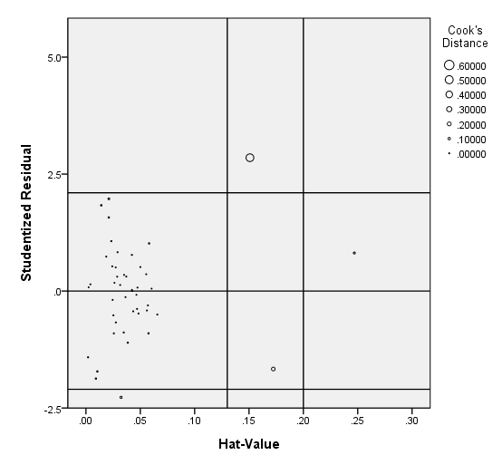
page 285 Figure 11.6 "Bubble plot" of Cook's D, studentized residuals, and hat values, for Duncan's regression of occupational prestige on income and education. Each point is plotted as a circle with area proportional to D. Horizontal reference lines are drawn at studentized residuals of 0 and +-2; vertical reference lines are drawn at values of 2h and 3h. Several observations are identified on the plot: Ministers and conductors have large hat values and relatively large residuals; reporters have a relatively large residual, but a small hat value; railroad engineers have a large hat value, but a small residual.
formats sre_1 (f4.1) lev_1 (f5.2) coo_1 (f7.5).

GGRAPH
  /GRAPHDATASET NAME="graphdataset" VARIABLES=LEV_1 sre_1 coo_1
  /GRAPHSPEC SOURCE=INLINE.
BEGIN GPL
  SOURCE: s=userSource(id("graphdataset"))
  DATA: LEV_1=col(source(s), name("LEV_1"))
  DATA: sre_1=col(source(s), name("sre_1"))
  DATA: COO_1=col(source(s), name("coo_1"))
  GUIDE: axis(dim(1), delta(.05), label("Hat-Value"))
  GUIDE: axis(dim(2), delta(2.5), label("Studentized Residual"))
GUIDE: legend(aesthetic(aesthetic.size), label("Cook's Distance"))
GUIDE: form.line(position(.2), color(color.black))
GUIDE: form.line(position(*, 0), color(color.black))
GUIDE: form.line(position(.13), color(color.black))
GUIDE: form.line(position(*, -2.1), color(color.black))
GUIDE: form.line(position(*, 2.1), color(color.black))
  SCALE: linear(dim(1), min(0), max(.3))
  SCALE: linear(dim(2), min(-2.5), max(5))
  ELEMENT: point(position(LEV_1*sre_1), size(COO_1))
END GPL.

page 288 Table 11.1 Data on the 1907 Romanian Peasant Rebellion: I, intensity of the rebellion (corrected from the original); C, commercialization of agriculture; T, traditionalism; M, market forces; and G, inequality of land tenure.
GET FILE='D:chirot.sav'.list county rebel agric trad market inequal.
COUNTY REBEL AGRIC TRAD MARKET INEQUAL1 -1.39 13.80 86.20 6.20 .60 2 .65 20.40 86.70 2.90 .72 3 1.89 27.60 79.30 16.90 .66 4 -.15 18.60 90.10 3.40 .74 5 -.86 17.20 84.50 9.00 .70 6 .11 21.50 81.50 5.20 .60 7 -.51 11.60 82.60 5.10 .52 8 -.86 20.40 82.40 6.30 .64 9 -.24 19.50 87.50 4.80 .68 10 -.77 8.90 85.60 9.50 .58 11 -.24 25.80 82.20 10.90 .68 12 -1.57 24.10 83.50 8.40 .74 13 -.51 22.00 88.30 6.20 .70 14 -1.57 24.20 84.90 6.10 .62 15 -.51 30.60 76.10 1.30 .76 16 -1.13 33.90 85.50 5.80 .70 17 -1.22 28.60 84.20 2.90 .58 18 -1.22 36.50 78.10 4.30 .72 19 -.86 40.90 84.40 2.30 .64 20 -1.39 6.80 76.30 3.60 .58 21 2.81 41.90 89.70 6.60 .66 22 -1.04 25.40 83.20 2.50 .68 23 1.57 30.50 80.20 4.10 .76 24 4.32 48.20 91.00 4.20 .70 25 3.79 46.00 90.50 3.70 .68 26 3.79 45.10 85.50 5.10 .64 27 -1.75 12.50 83.80 7.20 .50 28 .82 39.30 85.60 4.90 .60 29 2.59 47.70 87.60 5.20 .58 30 -.86 15.20 87.30 10.80 .42 31 -1.84 11.70 82.30 81.70 .42 32 -1.84 25.60 80.10 68.40 .26
Number of cases read: 32 Number of cases listed: 32
