page 297 Figure 12.1 The distribution of the studentized residuals from Ornstein’s interlocking-directorate regression. A normal quanitle comparison plot is shown in (a). The 95% confidence envelope is based on the standard errors of the order statistics for an independent normal sample. A nonparametric density estimate is shown in (b).
NOTE: The dummy variables need to be calculated before the graphs can be made.
NOTE: The q-q plot made by SPSS is rotated compared to the graph shown in the text.
GET FILE='D:/ornstein.sav'.

compute sec1 = 0.
if sector = "AGR" sec1 = 1.
compute sec2 = 0.
if sector = "BNK" sec2 = 1.
compute sec3 = 0.
if sector = "CON" sec3 = 1.
compute sec4 = 0.
if sector = "FIN" sec4 = 1.
compute sec5 = 0.
if sector = "HLD" sec5 = 1.
compute sec6 = 0.
if sector = "MAN" sec6 = 1.
compute sec7 = 0.
if sector = "MER" sec7 = 1.
compute sec8 = 0.
if sector = "MIN" sec8 = 1.
compute sec9 = 0.
if sector = "TRN" sec9 = 1.
compute sec10 = 0.
if sector = "WOD" sec10 = 1.
compute nat1 = 0.
if nation = "CAN" nat1 = 1.
compute nat2 = 0.
if nation = "OTH" nat2 = 1.
compute nat3 = 0.
if nation = "UK" nat3 = 1.
compute nat4 = 0.
if nation = "US" nat4 = 1.
compute asset1 = sqrt(assets).
execute.

regression
 /dep=intrlcks
 /method=enter asset1 nat2 nat3 nat4 sec1 sec2 sec3 sec4 sec5 sec7 sec8 sec9 sec10
 /save pre (pre_1) sre (sre_1).
pplot
/var = sre_1
/type = q-q
/dist=normal.
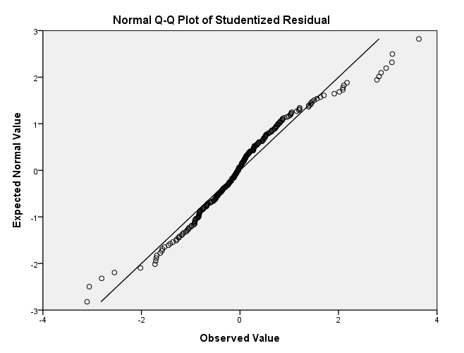
Panel b has been skipped for now.
page 298 Table 12.1 Regression of number of interlocking directorate and executive positions maintained by 248 dominant Canadian corporations on corporate assets, sector, and nation of control. The baseline category for sector is heavy manufacturing; for nation of control, Canada.
| Model | Variables Entered | Variables Removed | Method |
|---|---|---|---|
| 1 | SEC10, NAT2, SEC5, SEC2, SEC4, NAT3, SEC9, SEC3, SEC7, SEC1, NAT4, SEC8, ASSET1(a) | . | Enter |
| a All requested variables entered. | |||
| b Dependent Variable: Number interlocking director and executive positions | |||
| Model | R | R Square | Adjusted R Square | Std. Error of the Estimate |
|---|---|---|---|---|
| 1 | .809(a) | .655 | .635 | 9.712 |
| a Predictors: (Constant), SEC10, NAT2, SEC5, SEC2, SEC4, NAT3, SEC9, SEC3, SEC7, SEC1, NAT4, SEC8, ASSET1 | ||||
| b Dependent Variable: Number interlocking director and executive positions | ||||
| Model | Sum of Squares | df | Mean Square | F | Sig. | |
|---|---|---|---|---|---|---|
| 1 | Regression | 41816.553 | 13 | 3216.658 | 34.105 | .000(a) |
| Residual | 22069.834 | 234 | 94.316 | |
|
|
| Total | 63886.387 | 247 | |
|
|
|
| a Predictors: (Constant), SEC10, NAT2, SEC5, SEC2, SEC4, NAT3, SEC9, SEC3, SEC7, SEC1, NAT4, SEC8, ASSET1 | ||||||
| b Dependent Variable: Number interlocking director and executive positions | ||||||
| |
Unstandardized Coefficients | Standardized Coefficients | t | Sig. | ||
|---|---|---|---|---|---|---|
| Model | B | Std. Error | Beta | |||
| 1 | (Constant) | 4.190 | 1.846 | |
2.270 | .024 |
| ASSET1 | .252 | .019 | .849 | 13.594 | .000 | |
| NAT2 | -1.159 | 2.664 | -.019 | -.435 | .664 | |
| NAT3 | -4.444 | 2.649 | -.070 | -1.677 | .095 | |
| NAT4 | -8.089 | 1.481 | -.245 | -5.462 | .000 | |
| SEC1 | -1.200 | 2.040 | -.029 | -.588 | .557 | |
| SEC2 | -14.376 | 5.577 | -.158 | -2.578 | .011 | |
| SEC3 | -5.126 | 4.699 | -.045 | -1.091 | .276 | |
| SEC4 | -5.699 | 2.926 | -.101 | -1.948 | .053 | |
| SEC5 | -2.430 | 4.014 | -.025 | -.605 | .545 | |
| SEC7 | -.867 | 2.634 | -.015 | -.329 | .742 | |
| SEC8 | .342 | 2.012 | .009 | .170 | .865 | |
| SEC9 | -.381 | 2.820 | -.006 | -.135 | .893 | |
| SEC10 | 5.151 | 2.682 | .085 | 1.921 | .056 | |
| a Dependent Variable: Number interlocking director and executive positions | ||||||
| Case Number | Std. Residual | Number interlocking director and executive positions |
|---|---|---|
| 9 | 3.478 | 77 |
| 10 | -3.007 | 6 |
| 63 | 3.000 | 55 |
| 65 | 3.000 | 44 |
| a Dependent Variable: Number interlocking director and executive positions | ||
| |
Minimum | Maximum | Mean | Std. Deviation | N |
|---|---|---|---|---|---|
| Predicted Value | -1.57 | 86.57 | 13.58 | 13.011 | 248 |
| Std. Predicted Value | -1.165 | 5.610 | .000 | 1.000 | 248 |
| Standard Error of Predicted Value | 1.502 | 4.848 | 2.195 | .714 | 248 |
| Adjusted Predicted Value | -2.08 | 86.47 | 13.59 | 12.910 | 248 |
| Residual | -29.21 | 33.78 | .00 | 9.453 | 248 |
| Std. Residual | -3.007 | 3.478 | .000 | .973 | 248 |
| Stud. Residual | -3.104 | 3.632 | -.001 | 1.006 | 248 |
| Deleted Residual | -31.11 | 36.82 | -.01 | 10.113 | 248 |
| Stud. Deleted Residual | -3.163 | 3.731 | .001 | 1.015 | 248 |
| Mahal. Distance | 4.909 | 60.566 | 12.948 | 10.386 | 248 |
| Cook’s Distance | .000 | .119 | .005 | .013 | 248 |
| Centered Leverage Value | .020 | .245 | .052 | .042 | 248 |
| a Dependent Variable: Number interlocking director and executive positions | |||||
compute inter1 = sqrt(intrlcks + 1). execute.regression /dep=inter1 /method=enter asset1 nat2 nat3 nat4 sec1 sec2 sec3 sec4 sec5 sec7 sec8 sec9 sec10 /save sre_2.
| Model | Variables Entered | Variables Removed | Method |
|---|---|---|---|
| 1 | SEC10, NAT2, SEC5, SEC2, SEC4, NAT3, SEC9, SEC3, SEC7, SEC1, NAT4, SEC8, ASSET1(a) | . | Enter |
| a All requested variables entered. | |||
| b Dependent Variable: INTER1 | |||
| Model | R | R Square | Adjusted R Square | Std. Error of the Estimate |
|---|---|---|---|---|
| 1 | .762(a) | .580 | .557 | 1.21458 |
| a Predictors: (Constant), SEC10, NAT2, SEC5, SEC2, SEC4, NAT3, SEC9, SEC3, SEC7, SEC1, NAT4, SEC8, ASSET1 | ||||
| Model | Sum of Squares | df | Mean Square | F | Sig. | |
|---|---|---|---|---|---|---|
| 1 | Regression | 477.297 | 13 | 36.715 | 24.888 | .000(a) |
| Residual | 345.200 | 234 | 1.475 | |
|
|
| Total | 822.496 | 247 | |
|
|
|
| a Predictors: (Constant), SEC10, NAT2, SEC5, SEC2, SEC4, NAT3, SEC9, SEC3, SEC7, SEC1, NAT4, SEC8, ASSET1 | ||||||
| b Dependent Variable: INTER1 | ||||||
| |
Unstandardized Coefficients | Standardized Coefficients | t | Sig. | ||
|---|---|---|---|---|---|---|
| Model | B | Std. Error | Beta | |||
| 1 | (Constant) | 2.329 | .231 | |
10.089 | .000 |
| ASSET1 | 2.601E-02 | .002 | .773 | 11.229 | .000 | |
| NAT2 | -.114 | .333 | -.016 | -.342 | .733 | |
| NAT3 | -.527 | .331 | -.073 | -1.589 | .113 | |
| NAT4 | -1.105 | .185 | -.296 | -5.966 | .000 | |
| SEC1 | -5.672E-02 | .255 | -.012 | -.222 | .824 | |
| SEC2 | -2.251 | .697 | -.218 | -3.227 | .001 | |
| SEC3 | -.740 | .588 | -.057 | -1.259 | .209 | |
| SEC4 | -8.804E-02 | .366 | -.014 | -.241 | .810 | |
| SEC5 | -.245 | .502 | -.022 | -.489 | .626 | |
| SEC7 | .148 | .329 | .022 | .449 | .654 | |
| SEC8 | .356 | .252 | .081 | 1.416 | .158 | |
| SEC9 | .354 | .353 | .050 | 1.004 | .316 | |
| SEC10 | .786 | .335 | .115 | 2.343 | .020 | |
| a Dependent Variable: INTER1 | ||||||
page 299 Figure 12.2 The distribution of the studentized residuals from Orstein’s interlocking-directorate regression, after transforming the dependent variable. A normal quantile comparison plot is shown in (a), a nonparametric density estimate in (b).
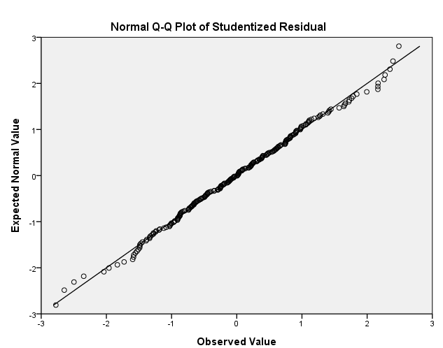
Panel b has been skipped for now.
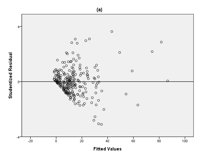
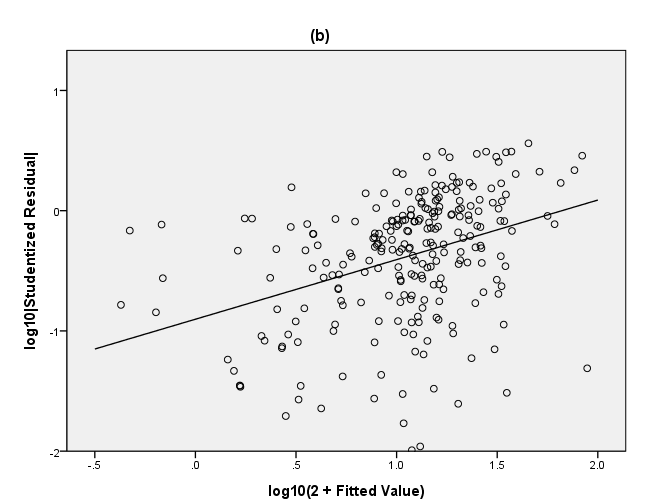
page 303 Figure 12.3 Detecting nonconstant spread in Ornstein’s interlocking-directorate regression. (a) A plot of studentized residuals versus fitted values. (b) A plot of log spread (log absolute studentized residuals) versus log level (log fitted values). The least-squares line is shown on the plot.
Panel (a)
GGRAPH
  /GRAPHDATASET NAME="graphdataset" VARIABLES=PRE_1 SRE_1
  /GRAPHSPEC SOURCE=INLINE.
BEGIN GPL
SOURCE: s=userSource(id("graphdataset"))
DATA: PRE_1=col(source(s), name("PRE_1"))
DATA: SRE_1=col(source(s), name("SRE_1"))
GUIDE: axis(dim(1), label("Fitted Values"), start(0.0), delta(20.0))
GUIDE: axis(dim(2), label("Studentized Residual"), start(0.0), delta(4.0))
GUIDE: text.title(label("(a)"))
GUIDE: form.line(position(*, 0), color(color.black))
SCALE: linear( dim( 1 ), min(-20), max(100) )
SCALE: linear( dim( 2 ), min(-4), max(4))
ELEMENT: point(position(PRE_1*SRE_1))
END GPL.
Panel (b)
compute abssre = abs(sre_1).
compute logsre = lg10(abssre).
compute logpre = lg10(pre_1 + 2).
execute.

formats logsre (f4.0) logpre (f4.1).
GGRAPH
  /GRAPHDATASET NAME="GraphDataset" VARIABLES= logpre logsre
  /GRAPHSPEC SOURCE=INLINE .
BEGIN GPL
SOURCE: s=userSource( id( "GraphDataset" ) )
DATA: logpre=col( source(s), name( "logpre" ) )
DATA:logsre=col( source(s), name( "logsre" ) )
GUIDE: text.title(label("(b)"))
GUIDE: axis( dim( 1 ), label( "log10(2 + Fitted Value)" ), start(0.0), delta(0.5) )
GUIDE: axis( dim( 2 ), label( "log10|Studentized Residual|" ), start(0.0), delta(1) )
SCALE: linear( dim( 1 ), min(-0.5), max(2) )
SCALE: linear( dim( 2 ), min(-2), max(1) )
ELEMENT: point( position(logpre * logsre ) )
ELEMENT: line(position(smooth.linear(logpre * logsre)))
END GPL.
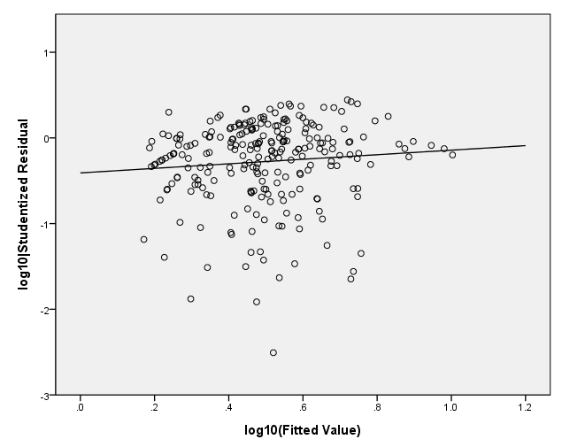
page 304 Figure 12.4 Plot of log spread versus log level for Ornstein's interlocking-directorate regression, after transforming the dependent variable. The least-squares line is shown on the plot.
regression
 /dep=inter1
 /method=enter asset1 nat2 nat3 nat4 sec1 sec2 sec3 sec4 sec5 sec7 sec8 sec9 sec10
 /save pre (pre_4) sre (sre_4).
| Model | Variables Entered | Variables Removed | Method |
|---|---|---|---|
| 1 | SEC10, NAT2, SEC5, SEC2, SEC4, NAT3, SEC9, SEC3, SEC7, SEC1, NAT4, SEC8, ASSET1(a) | . | Enter |
| a All requested variables entered. | |||
| b Dependent Variable: INTER1 | |||
| Model | R | R Square | Adjusted R Square | Std. Error of the Estimate |
|---|---|---|---|---|
| 1 | .762(a) | .580 | .557 | 1.21458 |
| a Predictors: (Constant), SEC10, NAT2, SEC5, SEC2, SEC4, NAT3, SEC9, SEC3, SEC7, SEC1, NAT4, SEC8, ASSET1 | ||||
| b Dependent Variable: INTER1 | ||||
| Model | Sum of Squares | df | Mean Square | F | Sig. | |
|---|---|---|---|---|---|---|
| 1 | Regression | 477.297 | 13 | 36.715 | 24.888 | .000(a) |
| Residual | 345.200 | 234 | 1.475 | |
|
|
| Total | 822.496 | 247 | |
|
|
|
| a Predictors: (Constant), SEC10, NAT2, SEC5, SEC2, SEC4, NAT3, SEC9, SEC3, SEC7, SEC1, NAT4, SEC8, ASSET1 | ||||||
| b Dependent Variable: INTER1 | ||||||
| |
Unstandardized Coefficients | Standardized Coefficients | t | Sig. | ||
|---|---|---|---|---|---|---|
| Model | B | Std. Error | Beta | |||
| 1 | (Constant) | 2.329 | .231 | |
10.089 | .000 |
| ASSET1 | 2.601E-02 | .002 | .773 | 11.229 | .000 | |
| NAT2 | -.114 | .333 | -.016 | -.342 | .733 | |
| NAT3 | -.527 | .331 | -.073 | -1.589 | .113 | |
| NAT4 | -1.105 | .185 | -.296 | -5.966 | .000 | |
| SEC1 | -5.672E-02 | .255 | -.012 | -.222 | .824 | |
| SEC2 | -2.251 | .697 | -.218 | -3.227 | .001 | |
| SEC3 | -.740 | .588 | -.057 | -1.259 | .209 | |
| SEC4 | -8.804E-02 | .366 | -.014 | -.241 | .810 | |
| SEC5 | -.245 | .502 | -.022 | -.489 | .626 | |
| SEC7 | .148 | .329 | .022 | .449 | .654 | |
| SEC8 | .356 | .252 | .081 | 1.416 | .158 | |
| SEC9 | .354 | .353 | .050 | 1.004 | .316 | |
| SEC10 | .786 | .335 | .115 | 2.343 | .020 | |
| a Dependent Variable: INTER1 | ||||||
| |
Minimum | Maximum | Mean | Std. Deviation | N |
|---|---|---|---|---|---|
| Predicted Value | 1.4829 | 10.0740 | 3.3562 | 1.39010 | 248 |
| Std. Predicted Value | -1.348 | 4.833 | .000 | 1.000 | 248 |
| Standard Error of Predicted Value | .18780 | .60637 | .27446 | .08935 | 248 |
| Adjusted Predicted Value | 1.5058 | 10.2327 | 3.3578 | 1.38810 | 248 |
| Residual | -3.2470 | 2.9809 | .0000 | 1.18219 | 248 |
| Std. Residual | -2.673 | 2.454 | .000 | .973 | 248 |
| Stud. Residual | -2.775 | 2.487 | -.001 | 1.001 | 248 |
| Deleted Residual | -3.4995 | 3.0611 | -.0016 | 1.25220 | 248 |
| Stud. Deleted Residual | -2.816 | 2.515 | .000 | 1.005 | 248 |
| Mahal. Distance | 4.909 | 60.566 | 12.948 | 10.386 | 248 |
| Cook's Distance | .000 | .051 | .004 | .007 | 248 |
| Centered Leverage Value | .020 | .245 | .052 | .042 | 248 |
| a Dependent Variable: INTER1 | |||||
compute logfit4 = lg10(pre_4).
compute abs4 = abs(sre_4).
compute logres4 = lg10(abs4).
execute.
regression
 /dep=logres4
 /method=enter logfit4.
| Model | Variables Entered | Variables Removed | Method |
|---|---|---|---|
| 1 | LOGFIT4(a) | . | Enter |
| a All requested variables entered. | |||
| b Dependent Variable: LOGRES4 | |||
| Model | R | R Square | Adjusted R Square | Std. Error of the Estimate |
|---|---|---|---|---|
| 1 | .089(a) | .008 | .004 | .48514 |
| a Predictors: (Constant), LOGFIT4 | ||||
| Model | Sum of Squares | df | Mean Square | F | Sig. | |
|---|---|---|---|---|---|---|
| 1 | Regression | .466 | 1 | .466 | 1.980 | .161(a) |
| Residual | 57.898 | 246 | .235 | |
|
|
| Total | 58.364 | 247 | |
|
|
|
| a Predictors: (Constant), LOGFIT4 | ||||||
| b Dependent Variable: LOGRES4 | ||||||
| |
Unstandardized Coefficients | Standardized Coefficients | t | Sig. | ||
|---|---|---|---|---|---|---|
| Model | B | Std. Error | Beta | |||
| 1 | (Constant) | -.408 | .098 | |
-4.161 | .000 |
| LOGFIT4 | .265 | .189 | .089 | 1.407 | .161 | |
| a Dependent Variable: LOGRES4 | ||||||
formats logres4 (f2.0) logfit4 (f3.1).
GGRAPH
  /GRAPHDATASET NAME="GraphDataset" VARIABLES= logres4 logfit4
  /GRAPHSPEC SOURCE=INLINE .
BEGIN GPL
SOURCE: s=userSource( id( "GraphDataset" ) )
DATA: logres4=col( source(s), name( "logres4" ) )
DATA: logfit4=col( source(s), name( "logfit4" ) )
GUIDE: axis( dim( 1 ), label( "log10(Fitted Value)" ), start(0.0), delta(.2) )
GUIDE: axis( dim( 2 ), label( "log10|Studentized Residual" ), start(0.0), delta(1) )
SCALE: linear( dim( 1 ), min(0), max(1.2) )
SCALE: linear( dim( 2 ), min(-3), max(1) )
ELEMENT: point( position( logfit4 * logres4 ) )
ELEMENT: line(position(smooth.linear(logfit4 * logres4)))
END GPL.
page 311 Figure 12.5 The residual plots of E versus X (in the lower panels) are identical, even though the regression of Y on X in (a) is nonmonotone while that in (b) is monotone.
NOTE: These graphs have been skipped for now.
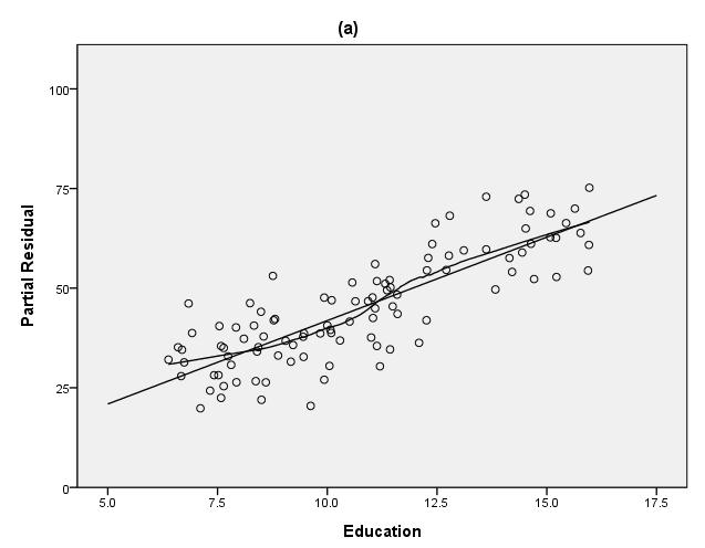
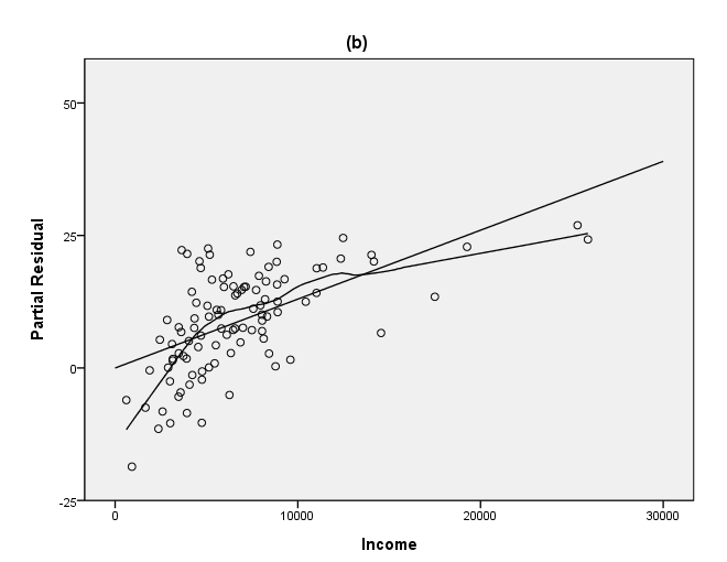
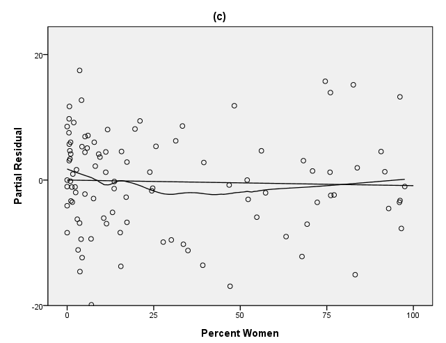
page 312 Figure 12.6 Partial-residual plots for the regression of occupational prestige on (a) education, (b) income, (c) percentage of women. The data are for 102 Canadian occupations in 1971. The least-squares line and a nonparamentric-regression smooth are shown on each plot.
GET FILE='D:prestige.sav'.

regression
 /dep=prestige
 /method=enter percwomn educat income
 /save res.
| Model | Variables Entered | Variables Removed | Method |
|---|---|---|---|
| 1 | Average income, dollars, % of incumbents who were women, Average education, years(a) | . | Enter |
| a All requested variables entered. | |||
| b Dependent Variable: Pineo-Porter prestige score occ. | |||
| Model | R | R Square | Adjusted R Square | Std. Error of the Estimate |
|---|---|---|---|---|
| 1 | .893(a) | .798 | .792 | 7.84647 |
| a Predictors: (Constant), Average income, dollars, % of incumbents who were women, Average education, years | ||||
| b Dependent Variable: Pineo-Porter prestige score occ. | ||||
| Model | Sum of Squares | df | Mean Square | F | Sig. | |
|---|---|---|---|---|---|---|
| 1 | Regression | 23861.856 | 3 | 7953.952 | 129.192 | .000(a) |
| Residual | 6033.570 | 98 | 61.567 | |
|
|
| Total | 29895.426 | 101 | |
|
|
|
| a Predictors: (Constant), Average income, dollars, % of incumbents who were women, Average education, years | ||||||
| b Dependent Variable: Pineo-Porter prestige score occ. | ||||||
| |
Unstandardized Coefficients | Standardized Coefficients | t | Sig. | ||
|---|---|---|---|---|---|---|
| Model | B | Std. Error | Beta | |||
| 1 | (Constant) | -6.794 | 3.239 | |
-2.098 | .039 |
| % of incumbents who were women | -8.905E-03 | .030 | -.016 | -.293 | .770 | |
| Average education, years | 4.187 | .389 | .664 | 10.771 | .000 | |
| Average income, dollars | 1.314E-03 | .000 | .324 | 4.729 | .000 | |
| a Dependent Variable: Pineo-Porter prestige score occ. | ||||||
| |
Minimum | Maximum | Mean | Std. Deviation | N |
|---|---|---|---|---|---|
| Predicted Value | 22.8487 | 93.1739 | 46.8333 | 15.37062 | 102 |
| Residual | -19.8246 | 17.5045 | .0000 | 7.72906 | 102 |
| Std. Predicted Value | -1.560 | 3.015 | .000 | 1.000 | 102 |
| Std. Residual | -2.527 | 2.231 | .000 | .985 | 102 |
| a Dependent Variable: Pineo-Porter prestige score occ. | |||||
NOTE: We need to look at the output and get the coefficient for the variable education to complete the necessary calculation.
Panel (a)
compute residu = res_1 + (4.187*educat).

formats residu (f3.0) educat (f4.1).
GGRAPH
  /GRAPHDATASET NAME="GraphDataset" VARIABLES= residu educat
  /GRAPHSPEC SOURCE=INLINE .
BEGIN GPL
SOURCE: s=userSource( id( "GraphDataset" ) )
DATA: residu=col( source(s), name( "residu" ) )
DATA: educat=col( source(s), name( "educat" ) )
GUIDE: text.title(label("(a)"))
GUIDE: axis( dim( 1 ), label( "Education" ), start(0.0), delta(2.5) )
GUIDE: axis( dim( 2 ), label( "Partial Residual" ), start(0.0), delta(25.0) )
SCALE: linear( dim( 1 ), min(5), max(17.5) )
SCALE: linear( dim( 2 ), min(0), max(100) )
ELEMENT: point( position( educat * residu ) )
ELEMENT: line(position(smooth.linear(educat * residu)))
ELEMENT: line(position(smooth.loess(educat * residu)))
END GPL.
Panel (b)
compute resedu2 = res_1 + (.0013*income).

formats residu2 (f4.0).

GGRAPH
  /GRAPHDATASET NAME="GraphDataset" VARIABLES= residu2 income
  /GRAPHSPEC SOURCE=INLINE.
BEGIN GPL
SOURCE: s=userSource( id( "GraphDataset" ) )
DATA: residu2=col( source(s), name( "residu2" ) )
DATA: income=col( source(s), name( "income" ) )
GUIDE: text.title(label("(b)"))
GUIDE: axis( dim( 1 ), label( "Income" ), start(0.0), delta(10000) )
GUIDE: axis( dim( 2 ), label( "Partial Residual" ), start(0.0), delta(25)  )
SCALE: linear( dim( 1 ), min(0), max(30000) )
SCALE: linear( dim( 2 ), min(-25), max(50) )
ELEMENT: point( position( income * residu2 ) )
ELEMENT: line(position(smooth.linear(income * residu2)))
ELEMENT: line(position(smooth.loess(income * residu2)))
END GPL.
Panel (c)
compute resedu3 = res_1 + (-.0089*percwomn).

formats residu3 percwomn (f4.0).

GGRAPH
  /GRAPHDATASET NAME="GraphDataset" VARIABLES= residu3 percwomn
  /GRAPHSPEC SOURCE=INLINE.
BEGIN GPL
SOURCE: s=userSource( id( "GraphDataset" ) )
DATA: residu3=col( source(s), name( "residu3" ) )
DATA: percwomn=col( source(s), name( "percwomn" ) )
GUIDE: text.title(label("(c)"))
GUIDE: axis( dim( 1 ), label( "Percent Women" ), start(0.0), delta(25) )
GUIDE: axis( dim( 2 ), label( "Partial Residual" ), start(0.0), delta(20))
SCALE: linear( dim( 1 ), min(0), max(100) )
SCALE: linear( dim( 2 ), min(-20), max(20) )
ELEMENT: point( position( percwomn * residu3 ) )
ELEMENT: line(position(smooth.linear(percwomn * residu3)))
ELEMENT: line(position(smooth.loess(percwomn * residu3)))
END GPL.
page 313 Formula in the middle of the page.
NOTE: The criteria=tolerance option needs to used in this example or else SPSS will throw out the variable edu2 because of low tolerance.
GET FILE='D:prestige.sav'.

compute loginc = lg10(income)/lg10(2).
compute edu2 = educat*educat.
compute edu3 = educat**3.
compute w2 = percwomn*percwomn.
execute.
regression
 /criteria=tolerance(0.0000001)
 /dep=prestige
 /method=enter loginc percwomn w2 educat edu2 edu3
 /save res (res_2).
| For models with dependent variable Pineo-Porter prestige score occ., the following variables have low tolerances: EDU2 |
| Model | Variables Entered | Variables Removed | Method |
|---|---|---|---|
| 1 | EDU3, W2, LOGINC, % of incumbents who were women, Average education, years, EDU2(a) | . | Enter |
| a All requested variables entered. | |||
| b Dependent Variable: Pineo-Porter prestige score occ. | |||
| Model | R | R Square | Adjusted R Square | Std. Error of the Estimate |
|---|---|---|---|---|
| 1 | .925(a) | .856 | .847 | 6.72135 |
| a Predictors: (Constant), EDU3, W2, LOGINC, % of incumbents who were women, Average education, years, EDU2 | ||||
| b Dependent Variable: Pineo-Porter prestige score occ. | ||||
| Model | Sum of Squares | df | Mean Square | F | Sig. | |
|---|---|---|---|---|---|---|
| 1 | Regression | 25603.648 | 6 | 4267.275 | 94.458 | .000(a) |
| Residual | 4291.778 | 95 | 45.177 | |
|
|
| Total | 29895.426 | 101 | |
|
|
|
| a Predictors: (Constant), EDU3, W2, LOGINC, % of incumbents who were women, Average education, years, EDU2 | ||||||
| b Dependent Variable: Pineo-Porter prestige score occ. | ||||||
| |
Unstandardized Coefficients | Standardized Coefficients | t | Sig. | ||
|---|---|---|---|---|---|---|
| Model | B | Std. Error | Beta | |||
| 1 | (Constant) | 20.838 | 56.900 | |
.366 | .715 |
| LOGINC | 8.783 | 1.273 | .436 | 6.901 | .000 | |
| % of incumbents who were women | -.179 | .085 | -.331 | -2.108 | .038 | |
| W2 | 2.500E-03 | .001 | .414 | 2.704 | .008 | |
| Average education, years | -29.920 | 15.252 | -4.745 | -1.962 | .053 | |
| EDU2 | 2.916 | 1.414 | 10.414 | 2.062 | .042 | |
| EDU3 | -8.068E-02 | .042 | -5.106 | -1.911 | .059 | |
| a Dependent Variable: Pineo-Porter prestige score occ. | ||||||
| |
Minimum | Maximum | Mean | Std. Deviation | N |
|---|---|---|---|---|---|
| Predicted Value | 16.3538 | 84.9538 | 46.8333 | 15.92173 | 102 |
| Residual | -13.9603 | 17.0921 | .0000 | 6.51865 | 102 |
| Std. Predicted Value | -1.914 | 2.394 | .000 | 1.000 | 102 |
| Std. Residual | -2.077 | 2.543 | .000 | .970 | 102 |
| a Dependent Variable: Pineo-Porter prestige score occ. | |||||
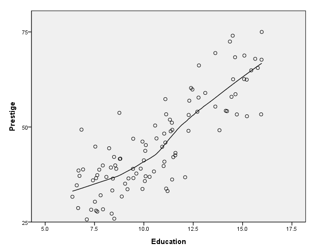
page 314 Figure 12.7 The partial relationship between prestige and education, holding income and percentage of women at their average levels. The curve shows the cubic fit for education. The points are partial residuals, obtained by adding the least-squares residuals to the education fit.
DESCRIPTIVES
  VARIABLES=income percwomn
  /STATISTICS=MEAN STDDEV MIN MAX.
| |
N | Minimum | Maximum | Mean | Std. Deviation |
|---|---|---|---|---|---|
| Average income, dollars | 102 | 611 | 25879 | 6797.90 | 4245.922 |
| % of incumbents who were women | 102 | .00 | 97.51 | 28.9790 | 31.72493 |
| Valid N (listwise) | 102 | |
|
|
|
compute pm = 20.8+8.78*lg10(6797.902)/lg10(2)-0.179*28.979+0.0025*28.979*28.979-29.9*educat+2.91*edu2-.0807*edu3.
compute pmr = res_2 + pm.
execute.
formats educat (f5.1) pmr (f3.0).

GGRAPH
  /GRAPHDATASET NAME="graphdataset" VARIABLES=educat pmr
  /GRAPHSPEC SOURCE=INLINE.
BEGIN GPL
SOURCE: s=userSource(id("graphdataset"))
DATA: educat=col(source(s), name("educat"))
DATA: pmr=col(source(s), name("pmr"))
GUIDE: axis(dim(1), label("Education"), start(0.0), delta(2.5))
GUIDE: axis(dim(2), label("Prestige"), start(0.0), delta(25))
SCALE: linear( dim( 1 ), min(5), max(17.5) )
SCALE: linear( dim( 2 ), min(25), max(75) )
ELEMENT: point(position(educat*pmr))
ELEMENT: line(position(smooth.loess(educat*pmr)))
END GPL.
page 319 Table 12.2 Analysis of variance for vocabulary test scores, showing the incremental F-test for nonlinearity of the relationship between vocabulary and education.
GET FILE='D:vocab.sav'.

regression
 /dep=vocab
 /method=enter educ.
| Model | Variables Entered | Variables Removed | Method |
|---|---|---|---|
| 1 | Years of Education(a) | . | Enter |
| a All requested variables entered. | |||
| b Dependent Variable: Vocabulary Test Score | |||
| Model | R | R Square | Adjusted R Square | Std. Error of the Estimate |
|---|---|---|---|---|
| 1 | .498(a) | .248 | .247 | 1.920 |
| a Predictors: (Constant), Years of Education | ||||
| Model | Sum of Squares | df | Mean Square | F | Sig. | |
|---|---|---|---|---|---|---|
| 1 | Regression | 1175.111 | 1 | 1175.111 | 318.917 | .000(a) |
| Residual | 3559.414 | 966 | 3.685 | |
|
|
| Total | 4734.525 | 967 | |
|
|
|
| a Predictors: (Constant), Years of Education | ||||||
| b Dependent Variable: Vocabulary Test Score | ||||||
| |
Unstandardized Coefficients | Standardized Coefficients | t | Sig. | ||
|---|---|---|---|---|---|---|
| Model | B | Std. Error | Beta | |||
| 1 | (Constant) | 1.135 | .276 | |
4.111 | .000 |
| Years of Education | .374 | .021 | .498 | 17.858 | .000 | |
| a Dependent Variable: Vocabulary Test Score | ||||||
NOTE: The do-loop below is needed in order to create the dummy variables.
DO REPEAT A=e1 e2 e3 e4 e5 e6 e7 e8 e9 e10 e11 e12 e13 e14 e15 e16 e17 e18 e19 e20
/B=1 2 3 4 5 6 7 8 9 10 11 12 13 14 15 16 17 18 19 20.
COMPUTE A=(educ=B).
END REPEAT.

regression
 /dep=vocab
 /method=enter e1 e2 e3 e4 e5 e6 e7 e8 e9 e10 e11 e12 e13 e14 e15 e16 e17 e18 e19 e20.
| For models with dependent variable Vocabulary Test Score, the following variables are constants or have missing correlations: E2. They will be deleted from the analysis. |
| Model | Variables Entered | Variables Removed | Method |
|---|---|---|---|
| 1 | E20, E1, E3, E5, E4, E6, E7, E19, E17, E9, E18, E10, E8, E15, E11, E13, E16, E14, E12(a) | . | Enter |
| a All requested variables entered. | |||
| b Dependent Variable: Vocabulary Test Score | |||
| Model | R | R Square | Adjusted R Square | Std. Error of the Estimate |
|---|---|---|---|---|
| 1 | .516(a) | .266 | .252 | 1.914 |
| a Predictors: (Constant), E20, E1, E3, E5, E4, E6, E7, E19, E17, E9, E18, E10, E8, E15, E11, E13, E16, E14, E12 | ||||
| Model | Sum of Squares | df | Mean Square | F | Sig. | |
|---|---|---|---|---|---|---|
| 1 | Regression | 1261.694 | 19 | 66.405 | 18.127 | .000(a) |
| Residual | 3472.831 | 948 | 3.663 | |
|
|
| Total | 4734.525 | 967 | |
|
|
|
| a Predictors: (Constant), E20, E1, E3, E5, E4, E6, E7, E19, E17, E9, E18, E10, E8, E15, E11, E13, E16, E14, E12 | ||||||
| b Dependent Variable: Vocabulary Test Score | ||||||
| |
Unstandardized Coefficients | Standardized Coefficients | t | Sig. | ||
|---|---|---|---|---|---|---|
| Model | B | Std. Error | Beta | |||
| 1 | (Constant) | 5.000 | 1.914 | |
2.612 | .009 |
| E1 | -4.000 | 2.707 | -.058 | -1.478 | .140 | |
| E3 | -3.000 | 2.344 | -.062 | -1.280 | .201 | |
| E4 | -2.833 | 2.067 | -.101 | -1.371 | .171 | |
| E5 | -2.500 | 2.140 | -.073 | -1.168 | .243 | |
| E6 | -1.714 | 2.046 | -.066 | -.838 | .402 | |
| E7 | -.818 | 1.999 | -.039 | -.409 | .682 | |
| E8 | -.682 | 1.936 | -.064 | -.352 | .725 | |
| E9 | -.765 | 1.942 | -.064 | -.394 | .694 | |
| E10 | -.561 | 1.937 | -.051 | -.290 | .772 | |
| E11 | -.328 | 1.930 | -.035 | -.170 | .865 | |
| E12 | .774 | 1.917 | .164 | .404 | .687 | |
| E13 | 1.308 | 1.926 | .161 | .679 | .497 | |
| E14 | 1.158 | 1.922 | .173 | .603 | .547 | |
| E15 | 1.673 | 1.933 | .166 | .866 | .387 | |
| E16 | 2.361 | 1.924 | .321 | 1.227 | .220 | |
| E17 | 2.419 | 1.945 | .193 | 1.244 | .214 | |
| E18 | 2.541 | 1.940 | .220 | 1.310 | .191 | |
| E19 | 3.692 | 1.986 | .192 | 1.859 | .063 | |
| E20 | 3.187 | 1.973 | .184 | 1.616 | .107 | |
| a Dependent Variable: Vocabulary Test Score | ||||||
NOTE: The nonlinear effect needs to be calculated by hand.
Sum of Squares for nonlinear effect: 1261.69399-1175.11129 = 86.5827 F-value: (86.57/18)/(3472.8/948) = 1.3128753 p-value: 17255134
page 324 Figure 12.8 Box-Cox transformations for Ornstein's interlocking-directorate regression. The maximized log likelihood is plotted against the transformation parameter lamda. The intersection of the line near the top of the graph with the log likelihood curve marks off the 95% confidence interval for lamda. The maximum of the log likelihood corresponds to the MLE of lamda.
NOTE: This figure has been skipped for now.
GET FILE='D:ornstein.sav'.

compute asset1 = sqrt(assets).
compute dep1 = (intrlcks + 1).
compute logy = ln(dep1).
compute c1 = mean(logy).
compute c = exp(c1).
NOTE: The mean of c = 8.2501268.
compute cv = dep1*(ln(dep1/8.2501268)-1).
execute.

compute sec1 = 0.
if sector = "AGR" sec1 = 1.
compute sec2 = 0.
if sector = "BNK" sec2 = 1.
compute sec3 = 0.
if sector = "CON" sec3 = 1.
compute sec4 = 0.
if sector = "FIN" sec4 = 1.
compute sec5 = 0.
if sector = "HLD" sec5 = 1.
compute sec6 = 0.
if sector = "MAN" sec6 = 1.
compute sec7 = 0.
if sector = "MER" sec7 = 1.
compute sec8 = 0.
if sector = "MIN" sec8 = 1.
compute sec9 = 0.
if sector = "TRN" sec9 = 1.
compute sec10 = 0.
if sector = "WOD" sec10 = 1.
compute nat1 = 0.
if nation = "CAN" nat1 = 1.
compute nat2 = 0.
if nation = "OTH" nat2 = 1.
compute nat3 = 0.
if nation = "UK" nat3 = 1.
compute nat4 = 0.
if nation = "US" nat4 = 1.
compute asset1 = sqrt(assets).
execute.

regression
 /dep=dep1
 /method=enter asset1 nat2 nat3 nat4 sec1 sec2 sec3 sec4 sec5 sec7 sec8 sec9 sec10
 /method=test(cv).
| Model | Variables Entered | Variables Removed | Method |
|---|---|---|---|
| 1 | SEC10, NAT2, SEC5, SEC2, SEC4, NAT3, SEC9, SEC3, SEC7, SEC1, NAT4, SEC8, ASSET1(a) | . | Enter |
| 2 | CV | . | Test |
| a All requested variables entered. | |||
| b Dependent Variable: DEP1 | |||
| Model | R | R Square | Adjusted R Square | Std. Error of the Estimate |
|---|---|---|---|---|
| 1 | .809(a) | .655 | .635 | 9.71162 |
| 2 | .928(b) | .862 | .853 | 6.15872 |
| a Predictors: (Constant), SEC10, NAT2, SEC5, SEC2, SEC4, NAT3, SEC9, SEC3, SEC7, SEC1, NAT4, SEC8, ASSET1 | ||||
| b Predictors: (Constant), SEC10, NAT2, SEC5, SEC2, SEC4, NAT3, SEC9, SEC3, SEC7, SEC1, NAT4, SEC8, ASSET1, CV | ||||
| Model | Sum of Squares | df | Mean Square | F | Sig. | R Square Change | ||
|---|---|---|---|---|---|---|---|---|
| 1 | Regression | 41816.553 | 13 | 3216.658 | 34.105 | .000(a) | |
|
| Residual | 22069.834 | 234 | 94.316 | |
|
|
||
| Total | 63886.387 | 247 | |
|
|
|
||
| 2 | Subset Tests | CV | 13232.181 | 1 | 13232.181 | 348.859 | .000(b) | .207 |
| Regression | 55048.734 | 14 | 3932.052 | 103.666 | .000(c) | |
||
| Residual | 8837.653 | 233 | 37.930 | |
|
|
||
| Total | 63886.387 | 247 | |
|
|
|
||
| a Predictors: (Constant), SEC10, NAT2, SEC5, SEC2, SEC4, NAT3, SEC9, SEC3, SEC7, SEC1, NAT4, SEC8, ASSET1 | ||||||||
| b Tested against the full model. | ||||||||
| c Predictors in the Full Model: (Constant), SEC10, NAT2, SEC5, SEC2, SEC4, NAT3, SEC9, SEC3, SEC7, SEC1, NAT4, SEC8, ASSET1, CV. | ||||||||
| d Dependent Variable: DEP1 | ||||||||
| |
Unstandardized Coefficients | Standardized Coefficients | t | Sig. | ||
|---|---|---|---|---|---|---|
| Model | B | Std. Error | Beta | |||
| 1 | (Constant) | 5.190 | 1.846 | |
2.812 | .005 |
| ASSET1 | .252 | .019 | .849 | 13.594 | .000 | |
| NAT2 | -1.159 | 2.664 | -.019 | -.435 | .664 | |
| NAT3 | -4.444 | 2.649 | -.070 | -1.677 | .095 | |
| NAT4 | -8.089 | 1.481 | -.245 | -5.462 | .000 | |
| SEC1 | -1.200 | 2.040 | -.029 | -.588 | .557 | |
| SEC2 | -14.376 | 5.577 | -.158 | -2.578 | .011 | |
| SEC3 | -5.126 | 4.699 | -.045 | -1.091 | .276 | |
| SEC4 | -5.699 | 2.926 | -.101 | -1.948 | .053 | |
| SEC5 | -2.430 | 4.014 | -.025 | -.605 | .545 | |
| SEC7 | -.867 | 2.634 | -.015 | -.329 | .742 | |
| SEC8 | .342 | 2.012 | .009 | .170 | .865 | |
| SEC9 | -.381 | 2.820 | -.006 | -.135 | .893 | |
| SEC10 | 5.151 | 2.682 | .085 | 1.921 | .056 | |
| 2 | (Constant) | 11.416 | 1.217 | |
9.379 | .000 |
| ASSET1 | 6.991E-02 | .015 | .236 | 4.582 | .000 | |
| NAT2 | -.137 | 1.690 | -.002 | -.081 | .935 | |
| NAT3 | -2.353 | 1.684 | -.037 | -1.397 | .164 | |
| NAT4 | -5.037 | .953 | -.153 | -5.283 | .000 | |
| SEC1 | -2.703E-02 | 1.295 | -.001 | -.021 | .983 | |
| SEC2 | -12.679 | 3.538 | -.140 | -3.584 | .000 | |
| SEC3 | -3.911 | 2.980 | -.034 | -1.312 | .191 | |
| SEC4 | 3.476 | 1.919 | .062 | 1.811 | .071 | |
| SEC5 | -.635 | 2.547 | -.007 | -.249 | .803 | |
| SEC7 | 1.511 | 1.675 | .026 | .902 | .368 | |
| SEC8 | 3.029 | 1.284 | .078 | 2.359 | .019 | |
| SEC9 | 3.208 | 1.798 | .052 | 1.784 | .076 | |
| SEC10 | 3.875 | 1.702 | .064 | 2.277 | .024 | |
| CV | .585 | .031 | .752 | 18.678 | .000 | |
| a Dependent Variable: DEP1 | ||||||
| |
Beta In | t | Sig. | Partial Correlation | Collinearity Statistics | |
|---|---|---|---|---|---|---|
| Model | Tolerance | |||||
| 1 | CV | .752(a) | 18.678 | .000 | .774 | .366 |
| a Predictors in the Model: (Constant), SEC10, NAT2, SEC5, SEC2, SEC4, NAT3, SEC9, SEC3, SEC7, SEC1, NAT4, SEC8, ASSET1 | ||||||
| b Dependent Variable: DEP1 | ||||||
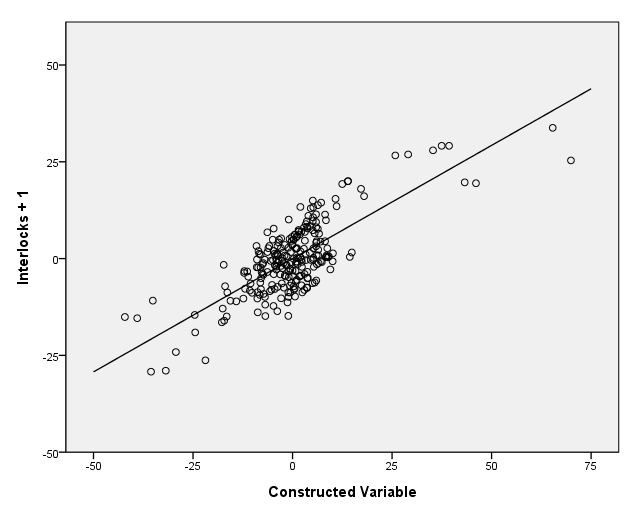
page 324 Figure 12.9 Constructed-variable plot for the Box-Cox . transformation of Ornstein's interlocking- directorate regression. The least-squares line is shown on the plot.
regression
 /dep=dep1
 /method=enter asset1 nat2 nat3 nat4 sec1 sec2 sec3 sec4 sec5 sec7 sec8 sec9 sec10
 /save res (res_1).
| Model | Variables Entered | Variables Removed | Method |
|---|---|---|---|
| 1 | SEC10, NAT2, SEC5, SEC2, SEC4, NAT3, SEC9, SEC3, SEC7, SEC1, NAT4, SEC8, ASSET1(a) | . | Enter |
| a All requested variables entered. | |||
| b Dependent Variable: DEP1 | |||
| Model | R | R Square | Adjusted R Square | Std. Error of the Estimate |
|---|---|---|---|---|
| 1 | .809(a) | .655 | .635 | 9.71162 |
| a Predictors: (Constant), SEC10, NAT2, SEC5, SEC2, SEC4, NAT3, SEC9, SEC3, SEC7, SEC1, NAT4, SEC8, ASSET1 | ||||
| b Dependent Variable: DEP1 | ||||
| Model | Sum of Squares | df | Mean Square | F | Sig. | |
|---|---|---|---|---|---|---|
| 1 | Regression | 41816.553 | 13 | 3216.658 | 34.105 | .000(a) |
| Residual | 22069.834 | 234 | 94.316 | |
|
|
| Total | 63886.387 | 247 | |
|
|
|
| a Predictors: (Constant), SEC10, NAT2, SEC5, SEC2, SEC4, NAT3, SEC9, SEC3, SEC7, SEC1, NAT4, SEC8, ASSET1 | ||||||
| b Dependent Variable: DEP1 | ||||||
| |
Unstandardized Coefficients | Standardized Coefficients | t | Sig. | ||
|---|---|---|---|---|---|---|
| Model | B | Std. Error | Beta | |||
| 1 | (Constant) | 5.190 | 1.846 | |
2.812 | .005 |
| ASSET1 | .252 | .019 | .849 | 13.594 | .000 | |
| NAT2 | -1.159 | 2.664 | -.019 | -.435 | .664 | |
| NAT3 | -4.444 | 2.649 | -.070 | -1.677 | .095 | |
| NAT4 | -8.089 | 1.481 | -.245 | -5.462 | .000 | |
| SEC1 | -1.200 | 2.040 | -.029 | -.588 | .557 | |
| SEC2 | -14.376 | 5.577 | -.158 | -2.578 | .011 | |
| SEC3 | -5.126 | 4.699 | -.045 | -1.091 | .276 | |
| SEC4 | -5.699 | 2.926 | -.101 | -1.948 | .053 | |
| SEC5 | -2.430 | 4.014 | -.025 | -.605 | .545 | |
| SEC7 | -.867 | 2.634 | -.015 | -.329 | .742 | |
| SEC8 | .342 | 2.012 | .009 | .170 | .865 | |
| SEC9 | -.381 | 2.820 | -.006 | -.135 | .893 | |
| SEC10 | 5.151 | 2.682 | .085 | 1.921 | .056 | |
| a Dependent Variable: DEP1 | ||||||
| Case Number | Std. Residual | DEP1 |
|---|---|---|
| 9 | 3.478 | 78.00 |
| 10 | -3.007 | 7.00 |
| 63 | 3.000 | 56.00 |
| 65 | 3.000 | 45.00 |
| a Dependent Variable: DEP1 | ||
| |
Minimum | Maximum | Mean | Std. Deviation | N |
|---|---|---|---|---|---|
| Predicted Value | -.5737 | 87.5717 | 14.5806 | 13.01145 | 248 |
| Residual | -29.2061 | 33.7793 | .0000 | 9.45260 | 248 |
| Std. Predicted Value | -1.165 | 5.610 | .000 | 1.000 | 248 |
| Std. Residual | -3.007 | 3.478 | .000 | .973 | 248 |
| a Dependent Variable: DEP1 | |||||
regression
 /dep=cv
 /method=enter asset1 nat2 nat3 nat4 sec1 sec2 sec3 sec4 sec5 sec7 sec8 sec9 sec10
 /save res (res_2).
| Model | Variables Entered | Variables Removed | Method |
|---|---|---|---|
| 1 | SEC10, NAT2, SEC5, SEC2, SEC4, NAT3, SEC9, SEC3, SEC7, SEC1, NAT4, SEC8, ASSET1(a) | . | Enter |
| a All requested variables entered. | |||
| b Dependent Variable: CV | |||
| Model | R | R Square | Adjusted R Square | Std. Error of the Estimate |
|---|---|---|---|---|
| 1 | .796(a) | .634 | .614 | 12.85360 |
| a Predictors: (Constant), SEC10, NAT2, SEC5, SEC2, SEC4, NAT3, SEC9, SEC3, SEC7, SEC1, NAT4, SEC8, ASSET1 | ||||
| b Dependent Variable: CV | ||||
| Model | Sum of Squares | df | Mean Square | F | Sig. | |
|---|---|---|---|---|---|---|
| 1 | Regression | 67034.519 | 13 | 5156.501 | 31.211 | .000(a) |
| Residual | 38660.348 | 234 | 165.215 | |
|
|
| Total | 105694.866 | 247 | |
|
|
|
| a Predictors: (Constant), SEC10, NAT2, SEC5, SEC2, SEC4, NAT3, SEC9, SEC3, SEC7, SEC1, NAT4, SEC8, ASSET1 | ||||||
| b Dependent Variable: CV | ||||||
| |
Unstandardized Coefficients | Standardized Coefficients | t | Sig. | ||
|---|---|---|---|---|---|---|
| Model | B | Std. Error | Beta | |||
| 1 | (Constant) | -10.642 | 2.443 | |
-4.355 | .000 |
| ASSET1 | .311 | .025 | .815 | 12.682 | .000 | |
| NAT2 | -1.746 | 3.526 | -.022 | -.495 | .621 | |
| NAT3 | -3.575 | 3.506 | -.044 | -1.019 | .309 | |
| NAT4 | -5.217 | 1.960 | -.123 | -2.662 | .008 | |
| SEC1 | -2.004 | 2.701 | -.038 | -.742 | .459 | |
| SEC2 | -2.901 | 7.381 | -.025 | -.393 | .695 | |
| SEC3 | -2.075 | 6.219 | -.014 | -.334 | .739 | |
| SEC4 | -15.683 | 3.872 | -.216 | -4.050 | .000 | |
| SEC5 | -3.068 | 5.313 | -.025 | -.577 | .564 | |
| SEC7 | -4.064 | 3.487 | -.054 | -1.166 | .245 | |
| SEC8 | -4.592 | 2.663 | -.092 | -1.724 | .086 | |
| SEC9 | -6.136 | 3.732 | -.077 | -1.644 | .102 | |
| SEC10 | 2.181 | 3.550 | .028 | .614 | .540 | |
| a Dependent Variable: CV | ||||||
| Case Number | Std. Residual | CV |
|---|---|---|
| 2 | 5.441 | 169.77 |
| 3 | 3.585 | 137.15 |
| 4 | -3.036 | 38.30 |
| 6 | 3.365 | 79.68 |
| 8 | -3.277 | -4.71 |
| 9 | 5.084 | 97.23 |
| 63 | 3.058 | 51.25 |
| a Dependent Variable: CV | ||
| |
Minimum | Maximum | Mean | Std. Deviation | N |
|---|---|---|---|---|---|
| Predicted Value | -18.0029 | 105.9243 | .5393 | 16.47406 | 248 |
| Residual | -42.1238 | 69.9304 | .0000 | 12.51078 | 248 |
| Std. Predicted Value | -1.126 | 6.397 | .000 | 1.000 | 248 |
| Std. Residual | -3.277 | 5.441 | .000 | .973 | 248 |
| a Dependent Variable: CV | |||||
regression
 /dep=res_1
 /method=enter res_2.
| Model | Variables Entered | Variables Removed | Method |
|---|---|---|---|
| 1 | Unstandardized Residual(a) | . | Enter |
| a All requested variables entered. | |||
| b Dependent Variable: Unstandardized Residual | |||
| Model | R | R Square | Adjusted R Square | Std. Error of the Estimate |
|---|---|---|---|---|
| 1 | .774(a) | .600 | .598 | 5.99378170 |
| a Predictors: (Constant), Unstandardized Residual | ||||
| Model | Sum of Squares | df | Mean Square | F | Sig. | |
|---|---|---|---|---|---|---|
| 1 | Regression | 13232.181 | 1 | 13232.181 | 368.324 | .000(a) |
| Residual | 8837.653 | 246 | 35.925 | |
|
|
| Total | 22069.834 | 247 | |
|
|
|
| a Predictors: (Constant), Unstandardized Residual | ||||||
| b Dependent Variable: Unstandardized Residual | ||||||
| |
Unstandardized Coefficients | Standardized Coefficients | t | Sig. | ||
|---|---|---|---|---|---|---|
| Model | B | Std. Error | Beta | |||
| 1 | (Constant) | 1.110E-14 | .381 | |
.000 | 1.000 |
| Unstandardized Residual | .585 | .030 | .774 | 19.192 | .000 | |
| a Dependent Variable: Unstandardized Residual | ||||||
formats res_1 res_2 (f3.0).
GGRAPH
  /GRAPHDATASET NAME="GraphDataset" VARIABLES= res_1 res_2
  /GRAPHSPEC SOURCE=INLINE.
BEGIN GPL
SOURCE: s=userSource( id( "GraphDataset" ) )
DATA: res_1=col( source(s), name( "res_1" ) )
DATA: res_2=col( source(s), name( "res_2" ) )
GUIDE: axis( dim( 1 ), label( "Constructed Variable" ), start(0.0), delta(25)  )
GUIDE: axis( dim( 2 ), label( "Interlocks + 1" ), start(0.0), delta(25) )
SCALE: linear( dim( 1 ), min(-50), max(75) )
SCALE: linear( dim( 2 ), min(-50), max(50) )
ELEMENT: point( position( res_2 * res_1 ) )
ELEMENT: line(position(smooth.linear(res_2 * res_1)))
END GPL.
page 325 at the bottom.
GET FILE='D:prestige.sav'.

compute w2 = percwomn**2.
compute linc = income*ln(income).
compute ledu = educat*ln(educat).
execute.
regression
 /dep=prestige
 /method=enter percwomn w2 educat income.
| Model | Variables Entered | Variables Removed | Method |
|---|---|---|---|
| 1 | Average income, dollars, W2, Average education, years, % of incumbents who were women(a) | . | Enter |
| a All requested variables entered. | |||
| b Dependent Variable: Pineo-Porter prestige score occ. | |||
| Model | R | R Square | Adjusted R Square | Std. Error of the Estimate |
|---|---|---|---|---|
| 1 | .896(a) | .802 | .794 | 7.80353 |
| a Predictors: (Constant), Average income, dollars, W2, Average education, years, % of incumbents who were women | ||||
| Model | Sum of Squares | df | Mean Square | F | Sig. | |
|---|---|---|---|---|---|---|
| 1 | Regression | 23988.605 | 4 | 5997.151 | 98.483 | .000(a) |
| Residual | 5906.821 | 97 | 60.895 | |
|
|
| Total | 29895.426 | 101 | |
|
|
|
| a Predictors: (Constant), Average income, dollars, W2, Average education, years, % of incumbents who were women | ||||||
| b Dependent Variable: Pineo-Porter prestige score occ. | ||||||
| |
Unstandardized Coefficients | Standardized Coefficients | t | Sig. | ||
|---|---|---|---|---|---|---|
| Model | B | Std. Error | Beta | |||
| 1 | (Constant) | -6.177 | 3.250 | |
-1.901 | .060 |
| % of incumbents who were women | -.145 | .099 | -.268 | -1.464 | .146 | |
| W2 | 1.538E-03 | .001 | .255 | 1.443 | .152 | |
| Average education, years | 4.260 | .390 | .676 | 10.926 | .000 | |
| Average income, dollars | 1.272E-03 | .000 | .314 | 4.579 | .000 | |
| a Dependent Variable: Pineo-Porter prestige score occ. | ||||||
compute b1 = 4.260.
compute b2 = .00127.
regression
 /dep=prestige
 /method=enter percwomn w2 educat income ledu linc.
| Model | Variables Entered | Variables Removed | Method |
|---|---|---|---|
| 1 | LINC, W2, Average education, years, % of incumbents who were women, Average income, dollars, LEDU(a) | . | Enter |
| a All requested variables entered. | |||
| b Dependent Variable: Pineo-Porter prestige score occ. | |||
| Model | R | R Square | Adjusted R Square | Std. Error of the Estimate |
|---|---|---|---|---|
| 1 | .923(a) | .853 | .843 | 6.81050 |
| a Predictors: (Constant), LINC, W2, Average education, years, % of incumbents who were women, Average income, dollars, LEDU | ||||
| Model | Sum of Squares | df | Mean Square | F | Sig. | |
|---|---|---|---|---|---|---|
| 1 | Regression | 25489.052 | 6 | 4248.175 | 91.589 | .000(a) |
| Residual | 4406.374 | 95 | 46.383 | |
|
|
| Total | 29895.426 | 101 | |
|
|
|
| a Predictors: (Constant), LINC, W2, Average education, years, % of incumbents who were women, Average income, dollars, LEDU | ||||||
| b Dependent Variable: Pineo-Porter prestige score occ. | ||||||
| |
Unstandardized Coefficients | Standardized Coefficients | t | Sig. | ||
|---|---|---|---|---|---|---|
| Model | B | Std. Error | Beta | |||
| 1 | (Constant) | 32.844 | 23.493 | |
1.398 | .165 |
| % of incumbents who were women | -.125 | .088 | -.230 | -1.413 | .161 | |
| W2 | 2.294E-03 | .001 | .380 | 2.418 | .018 | |
| Average education, years | -14.442 | 7.445 | -2.290 | -1.940 | .055 | |
| Average income, dollars | 2.648E-02 | .005 | 6.536 | 5.537 | .000 | |
| LEDU | 5.298 | 2.202 | 2.854 | 2.406 | .018 | |
| LINC | -2.430E-03 | .000 | -6.113 | -5.301 | .000 | |
| a Dependent Variable: Pineo-Porter prestige score occ. | ||||||
compute d1 = 5.298.
compute d2 = -.0024298.
NOTE: 1 + d1/b1 = 2.2435437. NOTE: 1 + d2/b2 = -.91030351.
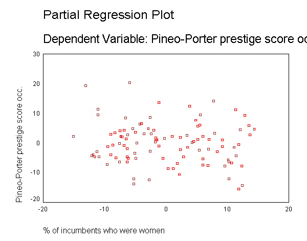
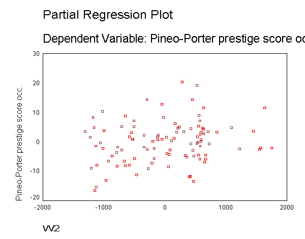
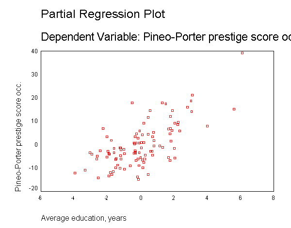
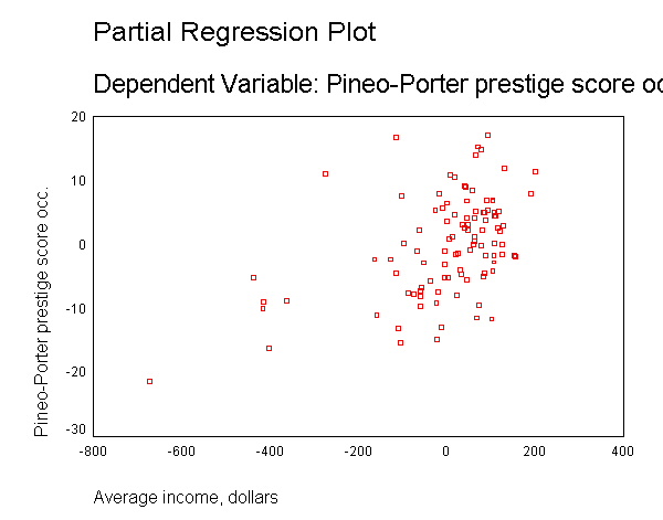
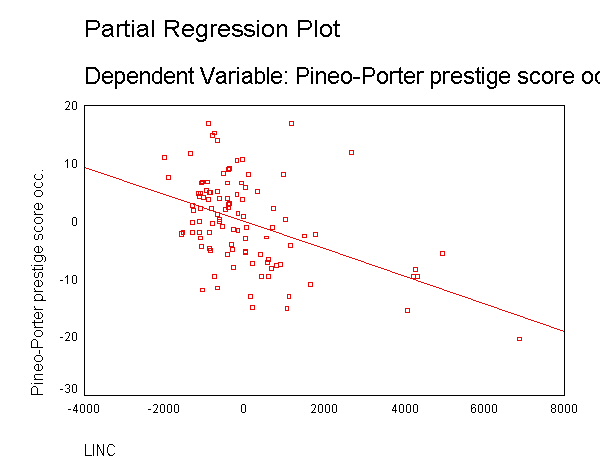
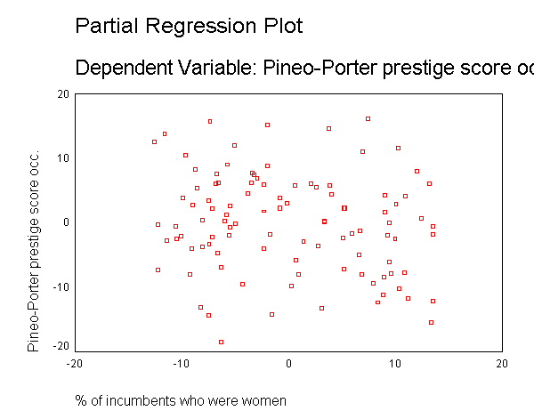
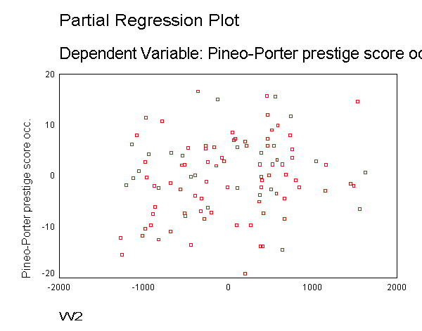
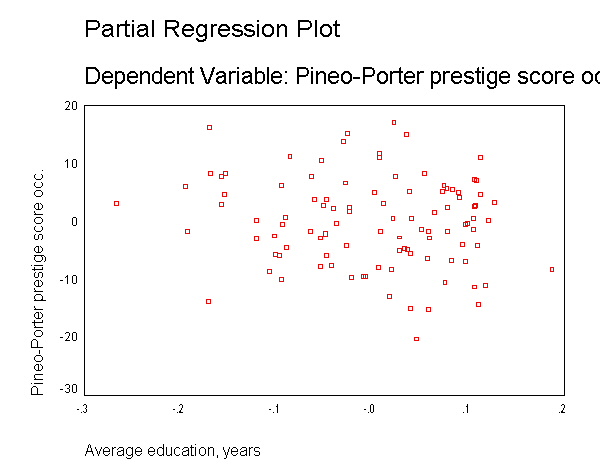
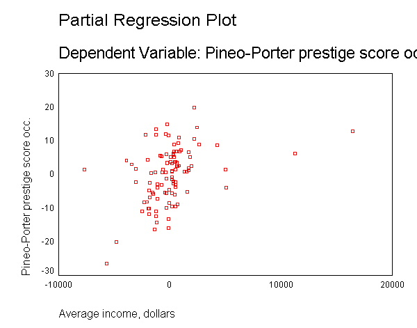
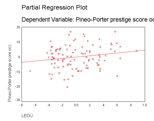
page 326 Figure 12.10 Constructed-variable plots for the Box-Tidwell transformation of (a) income and (b) education in the regression of occupational prestige on income, education, and percentage of women.
NOTE: To get the regression lines in the constructed variable plots, you need to double-click on the plot, go to chart, options and check on fit line total. Close the chart editor and the change will take effect.
NOTE: You cannot specify which partial plots you want: with SPSS code, it is all or nothing. However, only the last chart for each
regression is desired. Hence, only on those charts were the regression lines added.
Panel (a)
regression
 /dep=prestige
 /method=enter percwomn w2 educat income linc
 /partialplot all.
| Model | Variables Entered | Variables Removed | Method |
|---|---|---|---|
| 1 | LINC, W2, Average education, years, % of incumbents who were women, Average income, dollars(a) | . | Enter |
| a All requested variables entered. | |||
| b Dependent Variable: Pineo-Porter prestige score occ. | |||
| Model | R | R Square | Adjusted R Square | Std. Error of the Estimate |
|---|---|---|---|---|
| 1 | .918(a) | .844 | .835 | 6.97822 |
| a Predictors: (Constant), LINC, W2, Average education, years, % of incumbents who were women, Average income, dollars | ||||
| b Dependent Variable: Pineo-Porter prestige score occ. | ||||
| Model | Sum of Squares | df | Mean Square | F | Sig. | |
|---|---|---|---|---|---|---|
| 1 | Regression | 25220.648 | 5 | 5044.130 | 103.585 | .000(a) |
| Residual | 4674.778 | 96 | 48.696 | |
|
|
| Total | 29895.426 | 101 | |
|
|
|
| a Predictors: (Constant), LINC, W2, Average education, years, % of incumbents who were women, Average income, dollars | ||||||
| b Dependent Variable: Pineo-Porter prestige score occ. | ||||||
| |
Unstandardized Coefficients | Standardized Coefficients | t | Sig. | ||
|---|---|---|---|---|---|---|
| Model | B | Std. Error | Beta | |||
| 1 | (Constant) | -22.722 | 4.389 | |
-5.177 | .000 |
| % of incumbents who were women | -9.200E-02 | .089 | -.170 | -1.030 | .306 | |
| W2 | 1.875E-03 | .001 | .311 | 1.962 | .053 | |
| Average education, years | 3.444 | .385 | .546 | 8.957 | .000 | |
| Average income, dollars | 2.586E-02 | .005 | 6.381 | 5.283 | .000 | |
| LINC | -2.357E-03 | .000 | -5.931 | -5.030 | .000 | |
| a Dependent Variable: Pineo-Porter prestige score occ. | ||||||
| |
Minimum | Maximum | Mean | Std. Deviation | N |
|---|---|---|---|---|---|
| Predicted Value | 18.8346 | 81.2629 | 46.8333 | 15.80220 | 102 |
| Residual | -14.2740 | 19.7955 | .0000 | 6.80330 | 102 |
| Std. Predicted Value | -1.772 | 2.179 | .000 | 1.000 | 102 |
| Std. Residual | -2.046 | 2.837 | .000 | .975 | 102 |
| a Dependent Variable: Pineo-Porter prestige score occ. | |||||
Panel (b)
regression
 /dep=prestige
 /method=enter percwomn w2 educat income ledu
 /partialplot all.
| Model | Variables Entered | Variables Removed | Method |
|---|---|---|---|
| 1 | LEDU, W2, Average income, dollars, % of incumbents who were women, Average education, years(a) | . | Enter |
| a All requested variables entered. | |||
| b Dependent Variable: Pineo-Porter prestige score occ. | |||
| Model | R | R Square | Adjusted R Square | Std. Error of the Estimate |
|---|---|---|---|---|
| 1 | .899(a) | .809 | .799 | 7.71221 |
| a Predictors: (Constant), LEDU, W2, Average income, dollars, % of incumbents who were women, Average education, years | ||||
| b Dependent Variable: Pineo-Porter prestige score occ. | ||||
| Model | Sum of Squares | df | Mean Square | F | Sig. | |
|---|---|---|---|---|---|---|
| 1 | Regression | 24185.523 | 5 | 4837.105 | 81.326 | .000(a) |
| Residual | 5709.903 | 96 | 59.478 | |
|
|
| Total | 29895.426 | 101 | |
|
|
|
| a Predictors: (Constant), LEDU, W2, Average income, dollars, % of incumbents who were women, Average education, years | ||||||
| b Dependent Variable: Pineo-Porter prestige score occ. | ||||||
| |
Unstandardized Coefficients | Standardized Coefficients | t | Sig. | ||
|---|---|---|---|---|---|---|
| Model | B | Std. Error | Beta | |||
| 1 | (Constant) | 41.750 | 26.535 | |
1.573 | .119 |
| % of incumbents who were women | -.175 | .099 | -.322 | -1.757 | .082 | |
| W2 | 1.887E-03 | .001 | .312 | 1.762 | .081 | |
| Average education, years | -11.005 | 8.399 | -1.745 | -1.310 | .193 | |
| Average income, dollars | 1.161E-03 | .000 | .287 | 4.130 | .000 | |
| LEDU | 4.528 | 2.488 | 2.439 | 1.820 | .072 | |
| a Dependent Variable: Pineo-Porter prestige score occ. | ||||||
| |
Minimum | Maximum | Mean | Std. Deviation | N |
|---|---|---|---|---|---|
| Predicted Value | 25.9025 | 94.0397 | 46.8333 | 15.47452 | 102 |
| Residual | -19.6240 | 17.3239 | .0000 | 7.51889 | 102 |
| Std. Predicted Value | -1.353 | 3.051 | .000 | 1.000 | 102 |
| Std. Residual | -2.545 | 2.246 | .000 | .975 | 102 |
| a Dependent Variable: Pineo-Porter prestige score occ. | |||||
page 328 in the middle of the page.
GET FILE='D:AppsChristinesstuffARAornstein.sav'.compute sec1 = 0. if sector = "AGR" sec1 = 1. compute sec2 = 0. if sector = "BNK" sec2 = 1. compute sec3 = 0. if sector = "CON" sec3 = 1. compute sec4 = 0. if sector = "FIN" sec4 = 1. compute sec5 = 0. if sector = "HLD" sec5 = 1. compute sec6 = 0. if sector = "MAN" sec6 = 1. compute sec7 = 0. if sector = "MER" sec7 = 1. compute sec8 = 0. if sector = "MIN" sec8 = 1. compute sec9 = 0. if sector = "TRN" sec9 = 1. compute sec10 = 0. if sector = "WOD" sec10 = 1. compute nat1 = 0. if nation = "CAN" nat1 = 1. compute nat2 = 0. if nation = "OTH" nat2 = 1. compute nat3 = 0. if nation = "UK" nat3 = 1. compute nat4 = 0. if nation = "US" nat4 = 1. compute asset1 = sqrt(assets). compute y = intrlcks + 1. execute.
regression /dep=y /method=enter asset1 nat2 nat3 nat4 sec1 sec2 sec3 sec4 sec5 sec7 sec8 sec9 sec10 /save res pre.
| Model | Variables Entered | Variables Removed | Method |
|---|---|---|---|
| 1 | SEC10, NAT2, SEC5, SEC2, SEC4, NAT3, SEC9, SEC3, SEC7, SEC1, NAT4, SEC8, ASSET1(a) | . | Enter |
| a All requested variables entered. | |||
| b Dependent Variable: Y | |||
| Model | R | R Square | Adjusted R Square | Std. Error of the Estimate |
|---|---|---|---|---|
| 1 | .809(a) | .655 | .635 | 9.71162 |
| a Predictors: (Constant), SEC10, NAT2, SEC5, SEC2, SEC4, NAT3, SEC9, SEC3, SEC7, SEC1, NAT4, SEC8, ASSET1 | ||||
| b Dependent Variable: Y | ||||
| Model | Sum of Squares | df | Mean Square | F | Sig. | |
|---|---|---|---|---|---|---|
| 1 | Regression | 41816.553 | 13 | 3216.658 | 34.105 | .000(a) |
| Residual | 22069.834 | 234 | 94.316 | |
|
|
| Total | 63886.387 | 247 | |
|
|
|
| a Predictors: (Constant), SEC10, NAT2, SEC5, SEC2, SEC4, NAT3, SEC9, SEC3, SEC7, SEC1, NAT4, SEC8, ASSET1 | ||||||
| b Dependent Variable: Y | ||||||
| |
Unstandardized Coefficients | Standardized Coefficients | t | Sig. | ||
|---|---|---|---|---|---|---|
| Model | B | Std. Error | Beta | |||
| 1 | (Constant) | 5.190 | 1.846 | |
2.812 | .005 |
| ASSET1 | .252 | .019 | .849 | 13.594 | .000 | |
| NAT2 | -1.159 | 2.664 | -.019 | -.435 | .664 | |
| NAT3 | -4.444 | 2.649 | -.070 | -1.677 | .095 | |
| NAT4 | -8.089 | 1.481 | -.245 | -5.462 | .000 | |
| SEC1 | -1.200 | 2.040 | -.029 | -.588 | .557 | |
| SEC2 | -14.376 | 5.577 | -.158 | -2.578 | .011 | |
| SEC3 | -5.126 | 4.699 | -.045 | -1.091 | .276 | |
| SEC4 | -5.699 | 2.926 | -.101 | -1.948 | .053 | |
| SEC5 | -2.430 | 4.014 | -.025 | -.605 | .545 | |
| SEC7 | -.867 | 2.634 | -.015 | -.329 | .742 | |
| SEC8 | .342 | 2.012 | .009 | .170 | .865 | |
| SEC9 | -.381 | 2.820 | -.006 | -.135 | .893 | |
| SEC10 | 5.151 | 2.682 | .085 | 1.921 | .056 | |
| a Dependent Variable: Y | ||||||
| Case Number | Std. Residual | Y |
|---|---|---|
| 9 | 3.478 | 78.00 |
| 10 | -3.007 | 7.00 |
| 63 | 3.000 | 56.00 |
| 65 | 3.000 | 45.00 |
| a Dependent Variable: Y | ||
| |
Minimum | Maximum | Mean | Std. Deviation | N |
|---|---|---|---|---|---|
| Predicted Value | -.5737 | 87.5717 | 14.5806 | 13.01145 | 248 |
| Residual | -29.2061 | 33.7793 | .0000 | 9.45260 | 248 |
| Std. Predicted Value | -1.165 | 5.610 | .000 | 1.000 | 248 |
| Std. Residual | -3.007 | 3.478 | .000 | .973 | 248 |
| a Dependent Variable: Y | |||||
compute res2 = res_1**2. execute.DESCRIPTIVES VARIABLES=res2 /STATISTICS=MEAN.
| |
N | Mean |
|---|---|---|
| RES2 | 248 | 88.9913 |
| Valid N (listwise) | 248 | |
NOTE: The mean of res2 is 88.913.
compute m = 88.913. compute u = res2/m. execute.regression /dep=u /method=enter pre_1.
| Model | Variables Entered | Variables Removed | Method |
|---|---|---|---|
| 1 | Unstandardized Predicted Value(a) | . | Enter |
| a All requested variables entered. | |||
| b Dependent Variable: U | |||
| Model | R | R Square | Adjusted R Square | Std. Error of the Estimate |
|---|---|---|---|---|
| 1 | .396(a) | .157 | .153 | 1.79848 |
| a Predictors: (Constant), Unstandardized Predicted Value | ||||
| Model | Sum of Squares | df | Mean Square | F | Sig. | |
|---|---|---|---|---|---|---|
| 1 | Regression | 147.909 | 1 | 147.909 | 45.728 | .000(a) |
| Residual | 795.695 | 246 | 3.235 | |
|
|
| Total | 943.604 | 247 | |
|
|
|
| a Predictors: (Constant), Unstandardized Predicted Value | ||||||
| b Dependent Variable: U | ||||||
| |
Unstandardized Coefficients | Standardized Coefficients | t | Sig. | ||
|---|---|---|---|---|---|---|
| Model | B | Std. Error | Beta | |||
| 1 | (Constant) | .134 | .172 | |
.779 | .437 |
| Unstandardized Predicted Value | 5.947E-02 | .009 | .396 | 6.762 | .000 | |
| a Dependent Variable: U | ||||||
NOTE: The model sums of squares divided by 2 is 147.6488/2 = 73.8244.
DESCRIPTIVES
  VARIABLES=pre_1
  /STATISTICS=MEAN.
| |
N | Mean |
|---|---|---|
| Unstandardized Predicted Value | 248 | 14.5806452 |
| Valid N (listwise) | 248 | |
NOTE: The mean of pre_1 is 14.58. 1 - .5*.0594*14.58 = .566974.
regression
 /dep=u
 /method=enter asset1 nat2 nat3 nat4 sec1 sec2 sec3 sec4 sec5 sec7 sec8 sec9 sec10
 /save res pre.
| Model | Variables Entered | Variables Removed | Method |
|---|---|---|---|
| 1 | SEC10, NAT2, SEC5, SEC2, SEC4, NAT3, SEC9, SEC3, SEC7, SEC1, NAT4, SEC8, ASSET1(a) | . | Enter |
| a All requested variables entered. | |||
| b Dependent Variable: U | |||
| Model | R | R Square | Adjusted R Square | Std. Error of the Estimate |
|---|---|---|---|---|
| 1 | .428(a) | .183 | .138 | 1.81484 |
| a Predictors: (Constant), SEC10, NAT2, SEC5, SEC2, SEC4, NAT3, SEC9, SEC3, SEC7, SEC1, NAT4, SEC8, ASSET1 | ||||
| b Dependent Variable: U | ||||
| Model | Sum of Squares | df | Mean Square | F | Sig. | |
|---|---|---|---|---|---|---|
| 1 | Regression | 172.894 | 13 | 13.300 | 4.038 | .000(a) |
| Residual | 770.710 | 234 | 3.294 | |
|
|
| Total | 943.604 | 247 | |
|
|
|
| a Predictors: (Constant), SEC10, NAT2, SEC5, SEC2, SEC4, NAT3, SEC9, SEC3, SEC7, SEC1, NAT4, SEC8, ASSET1 | ||||||
| b Dependent Variable: U | ||||||
| |
Unstandardized Coefficients | Standardized Coefficients | t | Sig. | ||
|---|---|---|---|---|---|---|
| Model | B | Std. Error | Beta | |||
| 1 | (Constant) | .579 | .345 | |
1.678 | .095 |
| ASSET1 | 1.809E-02 | .003 | .502 | 5.227 | .000 | |
| NAT2 | -.149 | .498 | -.020 | -.300 | .764 | |
| NAT3 | -.915 | .495 | -.119 | -1.849 | .066 | |
| NAT4 | -.782 | .277 | -.195 | -2.825 | .005 | |
| SEC1 | 4.828E-03 | .381 | .001 | .013 | .990 | |
| SEC2 | -2.689 | 1.042 | -.244 | -2.581 | .010 | |
| SEC3 | -.779 | .878 | -.056 | -.887 | .376 | |
| SEC4 | -.991 | .547 | -.144 | -1.812 | .071 | |
| SEC5 | -.505 | .750 | -.043 | -.673 | .501 | |
| SEC7 | -.290 | .492 | -.041 | -.590 | .556 | |
| SEC8 | 8.885E-02 | .376 | .019 | .236 | .813 | |
| SEC9 | -.477 | .527 | -.063 | -.905 | .366 | |
| SEC10 | .540 | .501 | .074 | 1.078 | .282 | |
| a Dependent Variable: U | ||||||
| Case Number | Std. Residual | U |
|---|---|---|
| 9 | 5.455 | 12.83 |
| 10 | 3.814 | 9.59 |
| 23 | 3.688 | 9.43 |
| 63 | 3.991 | 9.55 |
| 65 | 4.840 | 9.55 |
| 83 | 3.687 | 8.79 |
| 86 | 3.552 | 7.99 |
| 143 | 3.816 | 8.14 |
| a Dependent Variable: U | ||
| |
Minimum | Maximum | Mean | Std. Deviation | N |
|---|---|---|---|---|---|
| Predicted Value | -.8232 | 4.8419 | 1.0009 | .83665 | 248 |
| Residual | -4.8399 | 9.8995 | .0000 | 1.76643 | 248 |
| Std. Predicted Value | -2.180 | 4.591 | .000 | 1.000 | 248 |
| Std. Residual | -2.667 | 5.455 | .000 | .973 | 248 |
| a Dependent Variable: U | |||||
