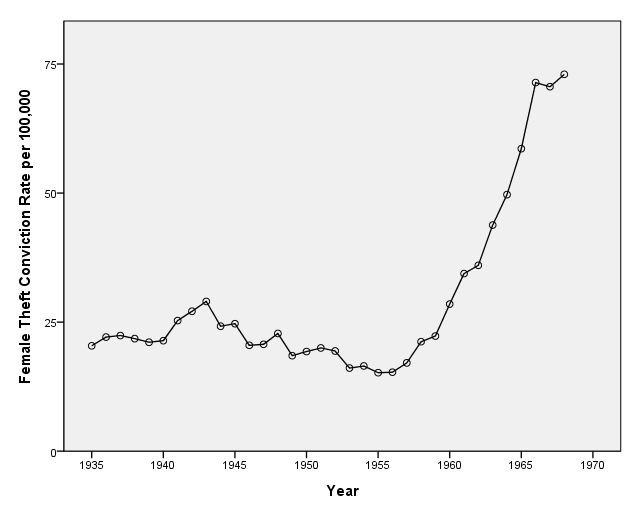
page 380 Figure 14.3 Canadian women’s theft conviction rate per 100,000 population, for the period 1935-1968.
GET FILE='D:hartnagl.sav'.

formats ftheft (f2.0).

GGRAPH
  /GRAPHDATASET NAME="graphdataset" VARIABLES=year ftheft
  /GRAPHSPEC SOURCE=INLINE.
BEGIN GPL
SOURCE: s=userSource(id("graphdataset"))
DATA: year=col(source(s), name("year"))
DATA: ftheft=col(source(s), name("ftheft"))
GUIDE: axis(dim(1), label("Year"), start(0.0), delta(5.0))
GUIDE: axis(dim(2), label("Female Theft Conviction Rate per 100,000"), start(0.0), delta(25.0))
SCALE: linear( dim( 1 ), min(1935), max(1970) )
SCALE: linear( dim( 2 ), min(0), max(75) )
ELEMENT: line(position(year*ftheft))
ELEMENT: point(position(year*ftheft))
END GPL.
page 380 Table 14.1 Regression of Canadian women's theft conviction rate on several independent variables, for the period 1935 to 1968: total fertility rate (TFR); labor force participation rate (LFPR); postsecondary degree rate (PSDR); and men's theft conviction rate (MRCR). The first set of EGLS estimates uses all 34 observations; the second set of EGLS estimates drops the first observation.
OLS
regression
 /dep=ftheft
 /method=enter fertil labor postsec mtheft
 /save res.
| Model | Variables Entered | Variables Removed | Method |
|---|---|---|---|
| 1 | Male Theft Conviction Rate per 100,000, Fertility Rate per 1000, Labor Force Participation Rate per 1000, Post Secondary Degree Rate per 1000(a) | . | Enter |
| a All requested variables entered. | |||
| b Dependent Variable: Female Theft Conviction Rate per 100,000 | |||
| Model | R | R Square | Adjusted R Square | Std. Error of the Estimate |
|---|---|---|---|---|
| 1 | .976(a) | .953 | .947 | 3.81245 |
| a Predictors: (Constant), Male Theft Conviction Rate per 100,000, Fertility Rate per 1000, Labor Force Participation Rate per 1000, Post Secondary Degree Rate per 1000 | ||||
| b Dependent Variable: Female Theft Conviction Rate per 100,000 | ||||
| Model | Sum of Squares | df | Mean Square | F | Sig. | |
|---|---|---|---|---|---|---|
| 1 | Regression | 8545.522 | 4 | 2136.380 | 146.984 | .000(a) |
| Residual | 421.509 | 29 | 14.535 | |
|
|
| Total | 8967.031 | 33 | |
|
|
|
| a Predictors: (Constant), Male Theft Conviction Rate per 100,000, Fertility Rate per 1000, Labor Force Participation Rate per 1000, Post Secondary Degree Rate per 1000 | ||||||
| b Dependent Variable: Female Theft Conviction Rate per 100,000 | ||||||
| |
Unstandardized Coefficients | Standardized Coefficients | t | Sig. | ||
|---|---|---|---|---|---|---|
| Model | B | Std. Error | Beta | |||
| 1 | (Constant) | -7.334 | 9.438 | |
-.777 | .443 |
| Fertility Rate per 1000 | -6.090E-03 | .001 | -.179 | -4.202 | .000 | |
| Labor Force Participation Rate per 1000 | .120 | .023 | .267 | 5.124 | .000 | |
| Post Secondary Degree Rate per 1000 | .552 | .043 | .684 | 12.753 | .000 | |
| Male Theft Conviction Rate per 100,000 | 3.932E-02 | .019 | .097 | 2.119 | .043 | |
| a Dependent Variable: Female Theft Conviction Rate per 100,000 | ||||||
| |
Minimum | Maximum | Mean | Std. Deviation | N |
|---|---|---|---|---|---|
| Predicted Value | 13.7209 | 79.0028 | 29.1294 | 16.09208 | 34 |
| Residual | -8.9739 | 7.1652 | .0000 | 3.57393 | 34 |
| Std. Predicted Value | -.958 | 3.099 | .000 | 1.000 | 34 |
| Std. Residual | -2.354 | 1.879 | .000 | .937 | 34 |
| a Dependent Variable: Female Theft Conviction Rate per 100,000 | |||||
EGLS(1)
ACF
  VARIABLES= res_1
  /NOLOG
  /MXAUTO 7
  /SERROR=IND.
MODEL:  MOD_4.

Variable:  RES_1        Missing cases:  4     Valid cases:  34

Autocorrelations:   RES_1   Unstandardized Residual

     Auto- Stand.
Lag  Corr.   Err. -1  -.75  -.5 -.25   0   .25  .5   .75   1   Box-Ljung  Prob.

  1   .244   .164               .       ***** .                    2.212   .137
  2  -.192   .162                . ****      .                     3.621   .164
  3  -.265   .159                .*****      .                     6.404   .094
  4   .000   .157                .     *     .                     6.404   .171
  5   .025   .154                .     *     .                     6.430   .267
  6   .017   .151                .     *     .                     6.442   .376
  7  -.149   .149                .  ***      .                     7.444   .384

Plot Symbols:      Autocorrelations *     Two Standard Error Limits .

Total cases:  38     Computable first lags:  33
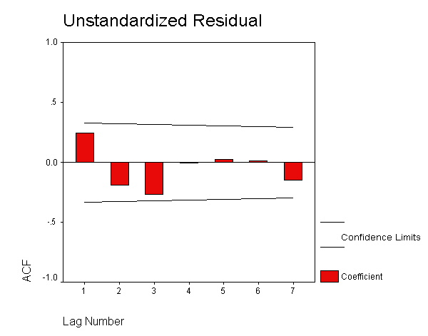
NOTE: The autocorrelation for the first lag is .2442.
compute fth1 = ftheft-0.244*lag(ftheft).  /*using transformation on page 378*/
compute fer1=fertil-0.244*lag(fertil).
compute lab1 =labor-0.244*lag(labor).
compute pos1 = postsec-0.244*lag(postsec).
compute mth1 =mtheft-0.244*lag(mtheft).
compute cons = .756.
if ($casenum=5) fth1 = sqrt(1-.244*.244)*ftheft.
if ($casenum=5) fer1 = sqrt(1-.244*.244)*fertil.
if ($casenum=5) lab1 = sqrt(1-.244*.244)*labor.
if ($casenum=5) pos1 = sqrt(1-.244*.244)*postsec.
if ($casenum=5) mth1 = sqrt(1-.244*.244)*mtheft.
if ($casenum=5) cons = sqrt(1-.244*.244).
execute.

regression
 /origin
 /dep=fth1
 /method=enter cons fer1 lab1 pos1 mth1.
| Model | Variables Entered | Variables Removed | Method |
|---|---|---|---|
| 1 | MTH1, POS1, FER1, LAB1, CONS(a) | . | Enter |
| a All requested variables entered. | |||
| b Dependent Variable: FTH1 | |||
| c Linear Regression through the Origin | |||
| Model | R | R Square(a) | Adjusted R Square | Std. Error of the Estimate |
|---|---|---|---|---|
| 1 | .991(b) | .983 | .980 | 3.66515 |
| a For regression through the origin (the no-intercept model), R Square measures the proportion of the variability in the dependent variable about the origin explained by regression. This CANNOT be compared to R Square for models which include an intercept. | ||||
| b Predictors: MTH1, POS1, FER1, LAB1, CONS | ||||
| Model | Sum of Squares | df | Mean Square | F | Sig. | |
|---|---|---|---|---|---|---|
| 1 | Regression | 22417.159 | 5 | 4483.432 | 333.755 | .000(a) |
| Residual | 389.566 | 29 | 13.433 | |
|
|
| Total | 22806.725(b) | 34 | |
|
|
|
| a Predictors: MTH1, POS1, FER1, LAB1, CONS | ||||||
| b This total sum of squares is not corrected for the constant because the constant is zero for regression through the origin. | ||||||
| c Dependent Variable: FTH1 | ||||||
| d Linear Regression through the Origin | ||||||
| |
Unstandardized Coefficients | Standardized Coefficients | t | Sig. | ||
|---|---|---|---|---|---|---|
| Model | B | Std. Error | Beta | |||
| 1 | CONS | -6.643 | 11.120 | -.196 | -.597 | .555 |
| FER1 | -5.879E-03 | .002 | -.575 | -3.305 | .003 | |
| LAB1 | .116 | .027 | .928 | 4.268 | .000 | |
| POS1 | .536 | .050 | .549 | 10.708 | .000 | |
| MTH1 | 3.993E-02 | .022 | .284 | 1.817 | .080 | |
| a Dependent Variable: FTH1 | ||||||
| b Linear Regression through the Origin | ||||||
EGLS(2)
filter off.
use 6 thru 38.
execute.

regression
 /origin
 /dep=fth1
 /method=enter cons fer1 lab1 pos1 mth1.
| Model | Variables Entered | Variables Removed | Method |
|---|---|---|---|
| 1 | MTH1, POS1, FER1, LAB1, CONS(a) | . | Enter |
| a All requested variables entered. | |||
| b Dependent Variable: FTH1 | |||
| c Linear Regression through the Origin | |||
| Model | R | R Square(a) | Adjusted R Square | Std. Error of the Estimate |
|---|---|---|---|---|
| 1 | .991(b) | .983 | .980 | 3.72183 |
| a For regression through the origin (the no-intercept model), R Square measures the proportion of the variability in the dependent variable about the origin explained by regression. This CANNOT be compared to R Square for models which include an intercept. | ||||
| b Predictors: MTH1, POS1, FER1, LAB1, CONS | ||||
| Model | Sum of Squares | df | Mean Square | F | Sig. | |
|---|---|---|---|---|---|---|
| 1 | Regression | 22027.486 | 5 | 4405.497 | 318.041 | .000(a) |
| Residual | 387.856 | 28 | 13.852 | |
|
|
| Total | 22415.342(b) | 33 | |
|
|
|
| a Predictors: MTH1, POS1, FER1, LAB1, CONS | ||||||
| b This total sum of squares is not corrected for the constant because the constant is zero for regression through the origin. | ||||||
| c Dependent Variable: FTH1 | ||||||
| d Linear Regression through the Origin | ||||||
| |
Unstandardized Coefficients | Standardized Coefficients | t | Sig. | ||
|---|---|---|---|---|---|---|
| Model | B | Std. Error | Beta | |||
| 1 | CONS | -5.519 | 11.737 | -.160 | -.470 | .642 |
| FER1 | -6.080E-03 | .002 | -.590 | -3.210 | .003 | |
| LAB1 | .114 | .028 | .904 | 4.047 | .000 | |
| POS1 | .534 | .051 | .550 | 10.466 | .000 | |
| MTH1 | 4.071E-02 | .022 | .285 | 1.815 | .080 | |
| a Dependent Variable: FTH1 | ||||||
| b Linear Regression through the Origin | ||||||
page 381 Figure 14.4 Residuals from the OLS regression of women's theft conviction rate on several independent variables.
tsplot variables = res_1
 /id = year
 /nolog
 /format nofill reference.

MODEL:  MOD_5.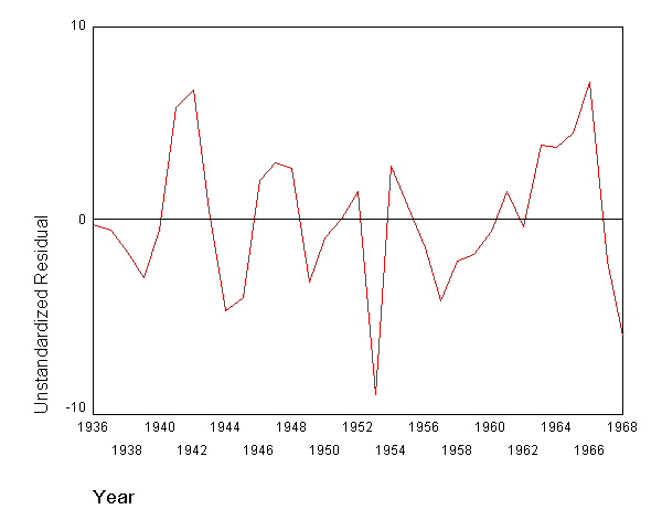
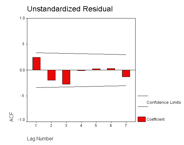
page 382 Figure 14.5 Residual autocorrelations from the OLS regression of women's theft conviction rates on several independent variables. The horizontal lines are at 0 and +-2 approximate standard errors.
ACF
  VARIABLES= res_1
  /NOLOG
  /MXAUTO 7
  /SERROR=IND.
MODEL:  MOD_6.

Autocorrelations:   RES_1   Unstandardized Residual

     Auto- Stand.
Lag  Corr.   Err. -1  -.75  -.5 -.25   0   .25  .5   .75   1   Box-Ljung  Prob.

  1   .244   .166               .       ***** .                    2.144   .143
  2  -.194   .164               .  ****       .                    3.552   .169
  3  -.271   .161                .*****      .                     6.369   .095
  4  -.008   .158                .     *     .                     6.371   .173
  5   .024   .156                .     *     .                     6.394   .270
  6   .032   .153                .      *    .                     6.437   .376
  7  -.131   .150                .  ***      .                     7.203   .408

Plot Symbols:      Autocorrelations *     Two Standard Error Limits .

Total cases:  33     Computable first lags:  32
page 399 Table 14.2 Population of the United States, in millions, 1790-1990.
GET FILE='D:us-pop.sav'.
list year pop.

     YEAR       POP

     1790      3.93
     1800      5.31
     1810      7.24
     1820      9.64
     1830     12.87
     1840     17.07
     1850     23.19
     1860     31.44
     1870     39.82
     1880     50.16
     1890     62.95
     1900     76.00
     1910     91.97
     1920    105.71
     1930    122.78
     1940    131.67
     1950    150.70
     1960    179.32
     1970    203.30
     1980    226.54
     1990    248.71

Number of cases read:  21    Number of cases listed:  21
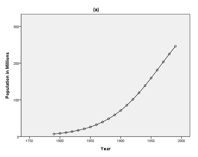
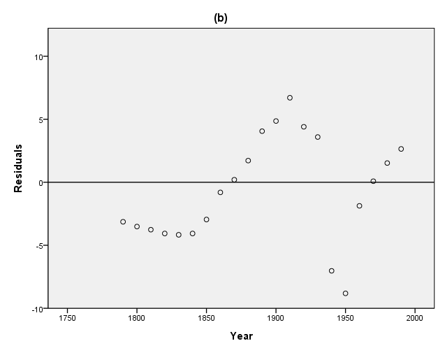
page 400 Figure 14.9 Panel (a) shows the population of the United States from 1790 through 1990; the line represents the fitted logistic growth model. Residuals from the logistic growth model are plotted against time in panel (b).
compute myear = year - 1790.
execute.
NOTE: The model is Y = b1/(1 + exp(-b2*(X-b3))).
model program b1 = 350 b2 = .3 b3 = 15.
compute pred = b1/(1 + exp(-b2*(myear-b3))) .
nlr pop /save pred resid.

All the derivatives will be calculated numerically.

The following new variables are being created:

Name          Label

PRED          Predicted Values
RESID         Residuals


 Iteration  Residual SS          B1          B2          B3

     1      1312135.325  350.000000  .300000000  15.0000000
     1.1    100157.1798  100.435896  .146786774  18.0029445
     2      100157.1798  100.435896  .146786774  18.0029445
     2.1    314792.0424  108.967416  -.19655968  37.0782489
     2.2    301359.2381  105.284961  -.15175500  26.9039676
     2.3    96429.25332  100.305195  .093343940  18.3767624
     3      96429.25332  100.305195  .093343940  18.3767624
     3.1    113742.0106  101.936425  .005176064  18.9207181
     3.2    94592.41883  100.419596  .077744762  18.4418469
     4      94592.41883  100.419596  .077744762  18.4418469
     4.1    89669.44906  100.864638  .052037091  18.5681848
     5      89669.44906  100.864638  .052037091  18.5681848
     5.1    80711.39660  102.880241  .020214578  18.7917751
     6      80711.39660  102.880241  .020214578  18.7917751
     6.1    75761.30175  117.004359  .016667397  19.6920945
     7      75761.30175  117.004359  .016667397  19.6920945
     7.1    71329.26105  125.989041  .018832793  25.4549182
     8      71329.26105  125.989041  .018832793  25.4549182
     8.1    68126.93436  138.787646  .013482007  37.2700619
     9      68126.93436  138.787646  .013482007  37.2700619
     9.1    72026.92171  100.475331  .037261255  42.1331140
     9.2    63743.31292  124.745379  .026231247  38.7300148
    10      63743.31292  124.745379  .026231247  38.7300148
    10.1    60371.83427  133.485133  .020449860  43.3845176
    11      60371.83427  133.485133  .020449860  43.3845176
    11.1    56267.71992  132.732592  .027346079  48.1835689
    12      56267.71992  132.732592  .027346079  48.1835689
    12.1    49140.29896  142.947629  .022777747  58.6348198
    13      49140.29896  142.947629  .022777747  58.6348198
    13.1    30900.04519  151.434468  .031779839  80.1714005
    14      30900.04519  151.434468  .031779839  80.1714005
    14.1    18286.94843  201.327451  .020421669  122.589280
    15      18286.94843  201.327451  .020421669  122.589280
    15.1    7706.823633  284.259383  .025776237  163.309783
    16      7706.823633  284.259383  .025776237  163.309783
    16.1    604.5219428  382.090975  .021506139  176.849371
    17      604.5219428  382.090975  .021506139  176.849371
    17.1    357.5474140  384.769943  .022823669  174.902732
    18      357.5474140  384.769943  .022823669  174.902732
    18.1    356.4069470  389.097381  .022656078  176.073140
    19      356.4069470  389.097381  .022656078  176.073140
    19.1    356.4000116  389.127490  .022663430  176.071884
    20      356.4000116  389.127490  .022663430  176.071884
    20.1    356.3999746  389.167013  .022661896  176.081370
    21      356.3999746  389.167013  .022661896  176.081370
    21.1    356.3999744  389.165419  .022661995  176.080966

Run stopped after 46 model evaluations and 21 derivative evaluations.
Iterations have been stopped because the relative reduction between successive
residual sums of squares is at most SSCON = 1.000E-08


Nonlinear Regression Summary Statistics     Dependent Variable POP

  Source                 DF  Sum of Squares  Mean Square

  Regression              3   277074.79529    92358.26510
  Residual               18      356.39997       19.80000
  Uncorrected Total      21   277431.19527

  (Corrected Total)      20   123093.52853

  R squared = 1 - Residual SS / Corrected SS =     .99710

                                           Asymptotic 95 %
                          Asymptotic     Confidence Interval
  Parameter   Estimate    Std. Error     Lower         Upper

  B1        389.16541926 30.812361782 324.43104928 453.89978924
  B2          .022661995   .001085690   .020381046   .024942945
  B3        176.08096572  7.244756710 160.86029667 191.30163477

  Asymptotic Correlation Matrix of the Parameter Estimates

                  B1        B2        B3

  B1          1.0000    -.9145     .9937
  B2          -.9145    1.0000    -.9328
  B3           .9937    -.9328    1.0000
formats pred (f3.0).

GGRAPH
  /GRAPHDATASET NAME="graphdataset" VARIABLES=year pred
  /GRAPHSPEC SOURCE=INLINE.
BEGIN GPL
SOURCE: s=userSource(id("graphdataset"))
DATA: year=col(source(s), name("year"))
DATA: pred=col(source(s), name("pred"))
GUIDE: axis(dim(1), label("Year"), start(0.0), delta(50.0))
GUIDE: axis(dim(2), label("Population in Millions"), start(0.0), delta(100.0))
GUIDE: text.title(label("(a)"))
SCALE: linear(dim(1), min(1750), max(2000))
SCALE: linear(dim(2), min(0), max(300))
ELEMENT: line(position(year*pred))
ELEMENT: point(position(year*pred))
END GPL.
formats resid (f3.0).
GGRAPH
  /GRAPHDATASET NAME="graphdataset" VARIABLES=year resid
  /GRAPHSPEC SOURCE=INLINE.
BEGIN GPL
SOURCE: s=userSource(id("graphdataset"))
DATA: year=col(source(s), name("year"))
DATA: resid=col(source(s), name("resid"))
GUIDE: axis(dim(1), label("Year"))
GUIDE: axis(dim(2), label("Residuals"))
GUIDE: text.title(label("(b)"))
GUIDE: form.line(position(*, 0), color(color.black))
SCALE: linear(dim(1), min(1750), max(2000))
ELEMENT: point(position(year*resid))
END GPL.
page 401 Table 14.3 Gauss-Newton iterations for the logistic growth model fit to the U.S. population data. Estimated asymptotic standard errors are given below the final coefficient estimates.
NOTE: The remained of this chapter has been skipped for now.
