page 16 Figure 2.1 A scatterplot showing the relationship between income (in thousands of dollars) and education (in years) for the population of employed Canadians. The line connects the mean incomes at the different levels of education. The "data" are hypothetical.
NOTE: We cannot reproduce this graph because the data are hypothetical.
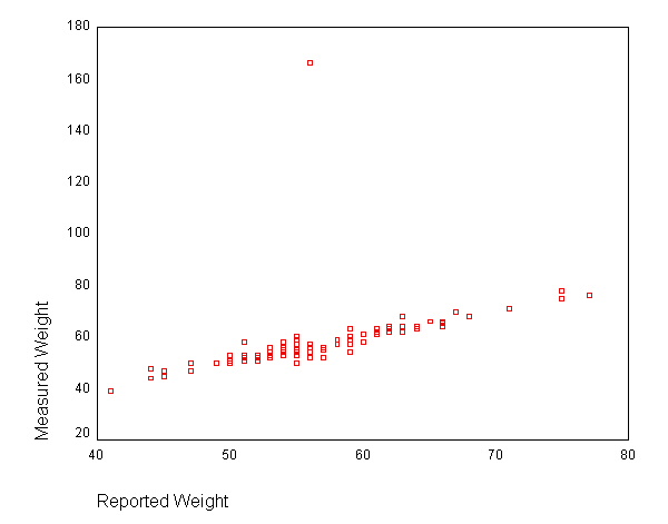
page 20 Figure 2.3 Native nonparametric regression of measured weight on reported weight, each in kilograms. The range of reported weight has been dissected into five intervals (separated by broken lines), each containing about 20 observations. The solid line connects the averages of measured weight and reported weight in the five intervals, shown as asterisks. The dotted line around which the points cluster is Y = X.
get file 'd:davis.sav'.USE ALL. COMPUTE filter_$=(female=1). VARIABLE LABEL filter_$ 'female=1 (FILTER)'. VALUE LABELS filter_$ 0 'Not Selected' 1 'Selected'. FORMAT filter_$ (f1.0). FILTER BY filter_$. EXECUTE.
GRAPH /SCATTERPLOT(BIVAR)=reptwt WITH measwt.

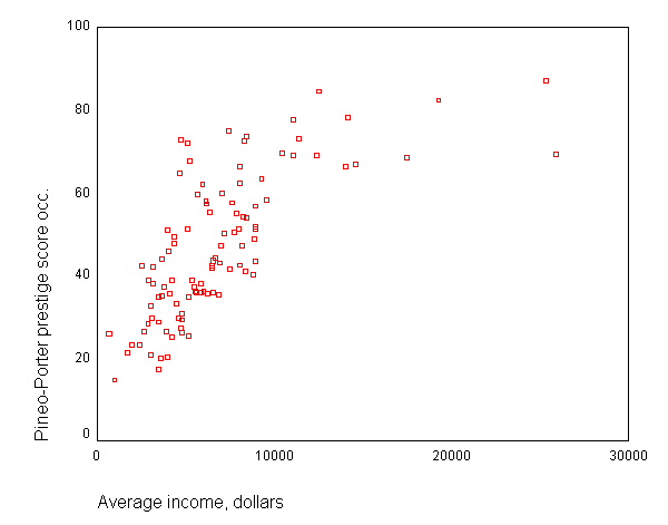
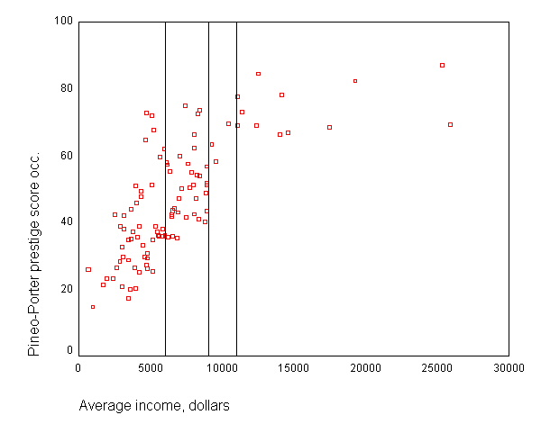
page 21 Figure 2.4 Naive nonparametric regression of occupational prestige on average income, for 102 Canadian occupations in 1971. The range of income has been dissected into five intervals, each containing about 20 observations. The line connects the average prestige and income scores in the five intervals, shown as asterisks.
NOTE: SPSS does not do band regression, so the lines cannot be added.
get file 'd:prestige.sav'.GRAPH /SCATTERPLOT(BIVAR)=income WITH prestige.

page 26 Figure 2.6 Nonparametric regression by local averaging for Davis's data on reported and measured weight. The data are shown by hollow dots, the local averages at each x-value by the line traced though the plot. Each local average is based on 20 of the 101 observations. Note the impact of the outlying observation on the averages that include it, and the flattening of the regression at the lowest and highest reported weights.
get file 'd:davis.sav'.USE ALL. COMPUTE filter_$=(female=1). VARIABLE LABEL filter_$ 'female=1 (FILTER)'. VALUE LABELS filter_$ 0 'Not Selected' 1 'Selected'. FORMAT filter_$ (f1.0). FILTER BY filter_$. EXECUTE.
GRAPH /SCATTERPLOT(BIVAR)=reptwt WITH measwt.

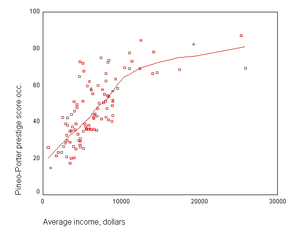
page 27 Figure 2.7 Nonparameteric regression of occupational prestige on income, using local averages. Each average includes 20 of the 102 observations; the averages are connected by a line.
get file 'd:prestige.sav'.GRAPH /SCATTERPLOT(BIVAR)=income WITH prestige.

page 28 Figure 2.8 Calculating locally weighted averages for the data on the prestige and income of Canadian occupations. Panels (a), (b) and (c) illustrate the calculation of the locally weighted average at x(80) = 8403: In panel (a), a window is defined enclosing the 40 nearest neighbors of x(80); panel (b) shows the tricube weight function centered at x(80); panel (c) shows the locally weighted average Y-value calculated at x(80). Panel (d) displays all 102 locally weighted averages connected by a line.
NOTE: To add the reference lines, use the code below and double-click on the resulting graph. From the menus at the top, choose chart and then reference line. Select x-axis and then OK. This will open up a dialogue box that will allow you to enter the values at which the reference lines should be placed. After adding the reference lines, click on OK. We know of no way to add the reference lines using code.
(a)
GRAPH
  /SCATTERPLOT(BIVAR)=income WITH prestige.

(b) We were unable to reproduce this graph.
(c) We were unable to reproduce this graph.
(d)
NOTE: To add the lowess smooth line, use the code below and double-click on the resulting graph. From the menus at the top, choose chart and then options. Single click on the fit line total box and then select fit options. Select lowess and click on continue and then OK. We know of no way to add the lowess smooth using code.
GRAPH
  /SCATTERPLOT(BIVAR)=income WITH prestige.

page 29 Figure 2.9 Locally weighted averages for the regression of measured weight on reported weight. Each average is based on 20 observations.
get file 'd:davis.sav'.USE ALL. COMPUTE filter_$=(female=1). VARIABLE LABEL filter_$ 'female=1 (FILTER)'. VALUE LABELS filter_$ 0 'Not Selected' 1 'Selected'. FORMAT filter_$ (f1.0). FILTER BY filter_$. EXECUTE.
GRAPH /SCATTERPLOT(BIVAR)=reptwt WITH measwt.

page 30 Figure 2.10 Robust regression for Davis's weight data by locally weighted averaging, downweighting outliers. Here, m = 20 observations are included in each local average, and the biweight tuning constant is t = 10. There is still some flattening of the regression curve at the lowest and highest X's.
We were unable to reproduce this graph using SPSS.
