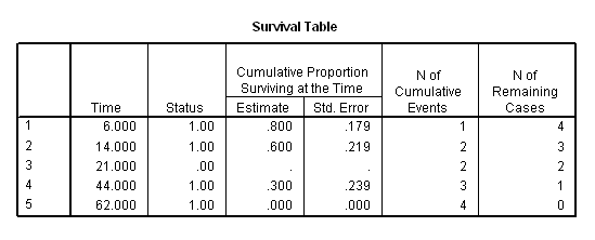
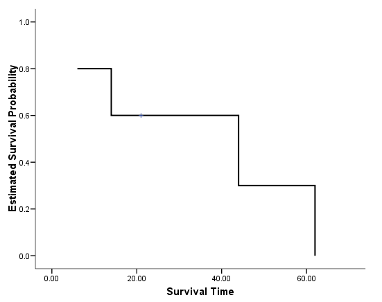
Table 2.1, Table 2.2 and Figure 2.1 on pages 17, 20, and 21.
data list free
/subject time censor.
begin data
  1 6  1
  2 44 1
  3 21 0
  4 14 1
  5 62 1
end data.

km time
 /status=censor(1)
 /plot survival .
Figure 2.2 on page 22. Instead of using the plot option on the km command, we saved the estimated survival probabilities and graph the function using the graph command to have more control over the graphics, such as the variable label of the y-axis.
get file='C:Dataasa2whas100.sav'.
compute time = foltime/365.25.
exe.
km time
/status=folstatus(1)
/print = none
/save survival(surv).
variable labels surv 'Estimated Survival Probability'.
variable labels time 'Survival Time (Years)'.
graph /scatterplot(bivar)=time with surv by folstatus.
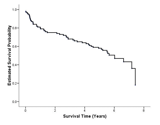
Note that the graphics editor has been used to produced the desired results, such as the background color, the left-join line style.
Table 2.3 on page 23.
km foltime
/status=folstatus(1)
/print = survival.

Table 2.4 on page 24. Note that we have manually deleted many columns from the output table.
survival table =time
/interval = thru 8 by 1
/status  = folstatus(1)
/print = table.
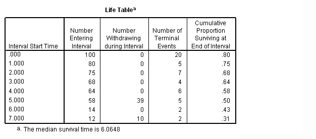
Figure 2.3 on page 25. Notice that the graph has be modified via chart editor.
survival table =time
/interval = thru 8 by 1
/status  = folstatus(1)
/plots (survival) = time.
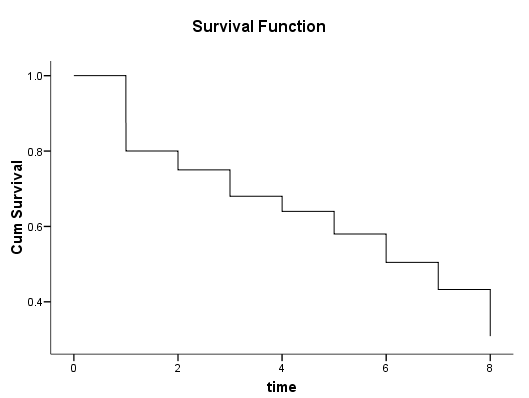
Figure 2.4 on page 26. This graph can be generated by using the chart editor to modify the graph above. Here are the main steps.
1) Double click on the graph to start the graphics editor.
2) Double click on the step line, then change the connecting method from Step to Straight.
3) Click Apply to confirm the change
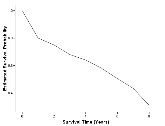
Figure 2.5 on page 31. In SPSS 15, the asymptotic standard error is calculated using Greenwood’s formula (see the SPSS manual on Algorithms for details.) Again, we have to rely on the SPSS chart editor to modify different aspects of the plot, such as adding the connecting lines, changing the legend and the background color.
get file='C:Dataasa2whas100.sav'.
compute time = foltime/365.25.
exe.
km time  /status=folstatus(1)
/print = none
/save survival(surv_km)  se(surv_se).

compute var2_6 = surv_se**2/(surv_km**2*(ln(surv_km))**2).
compute cl  =ln(-ln(surv_km)) - 1.96*sqrt(var2_6).
compute cu  =ln(-ln(surv_km)) + 1.96*sqrt(var2_6).
compute l = exp(-exp(cu)).
compute u = exp(-exp(cl)).
exe.

graph /scatterplot(overlay)=time time time with surv_km l u (pair).
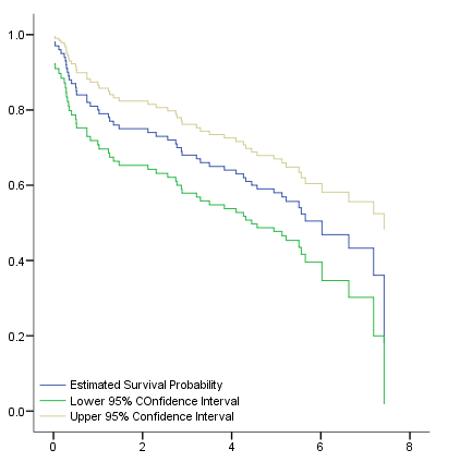
Figure 2.6 on page 32 shows the log-log, log, logit and arcsine transformations of the survival functions. Since SPSS does not provide these confidence interval variables, we will have to generate these variables via the compute command. The graph is produced with use of the chart editor.
get file='C:Dataasa2whas100.sav'.
compute time = foltime/365.25.
exe.
km time  /status=folstatus(1)
/print = none
/save survival(surv_km)  se(surv_se).

* log-log transformation.
compute ll_s = surv_se/(surv_km*ln(surv_km)).
compute ll_l  = exp(- exp(ln(-ln(surv_km))  -  1.96*ll_s)).
compute ll_u = exp(- exp(ln(-ln(surv_km))  + 1.96*ll_s)).
exe.

* log transformation, formula 2.3.
compute log_s = surv_se/surv_km.
compute log_l   = surv_km*exp( - 1.96*log_s).
compute log_u  = surv_km*exp(   1.96*log_s).
exe.

* logit transformation. f'=1/(S(t)*(1-S(t)).
compute logit_s = surv_se/(surv_km*(1-surv_km)).
compute logit_surv = ln(surv_km/(1-surv_km)).
compute logit_l   = exp(logit_surv  - 1.96*logit_s)/(1+exp(logit_surv   - 1.96*logit_s)).
compute logit_u  = exp(logit_surv  + 1.96*logit_s)/(1+exp(logit_surv + 1.96*logit_s)).
exe.

* arcsine transformation.
compute arcs_s = surv_se/sqrt(1-surv_km**2).
compute arcs_surv = arsin(surv_km).

compute arcs_l   = sine(arcs_surv  - 1.96*arcs_s).
compute arcs_u  = sine(arcs_surv + 1.96*arcs_s).
exe.

graph /scatterplot(overlay)=time time  time time time time time time time
       with surv_km ll_l ll_u log_l log_u logit_l logit_u arcs_l arcs_u  (pair).
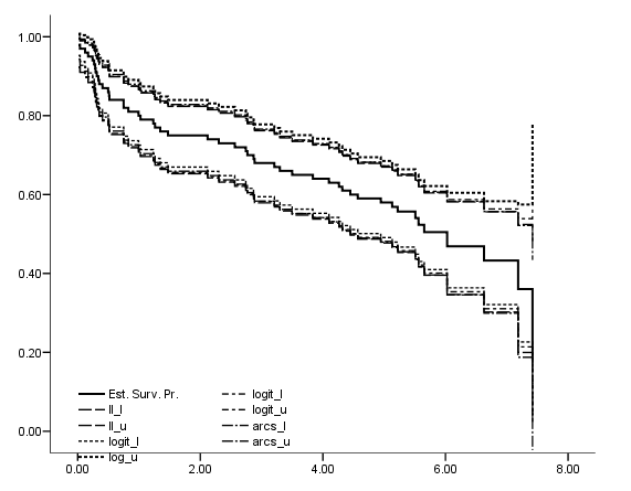
Figure 2.7 on page 34. The graph is produced with use of the chart editor.
get file='C:Dataasa2whas100.sav'.
compute time = foltime/365.25.

km time
/status=folstatus(1)
/save survival(surv_km) se(surv_se).
* compute the variance of the log of the Kaplan-Meier estimateor.
compute sigma2 = surv_se**2/surv_km**2.
exe.
* what is H_a_alpha in formula (2.9)?
* compute "a" first. Notice that the largest noncensored vlaue of time is 2710, or 7.42 years.
* n = 100 cases.
* notice the value for sigma2 when time = 7.42 is .557.
* a = 100*.557/(1+100*.557).
* looking up the table from Appendix 3: we get H = 1.358.
compute bl  = ln(-ln(surv_km)) - 1.358*(1+100*sigma2)/(sqrt(100)*ln(surv_km)).
compute bu  = ln(-ln(surv_km)) + 1.358*(1+100*sigma2)/(sqrt(100)*ln(surv_km)).
exe.
compute ebl  = exp(-exp(bu)).
compute ebu = exp(-exp(bl)).
compute var2_6 = surv_se**2/(surv_km**2*(ln(surv_km))**2).
compute cl  =ln(-ln(surv_km)) - 1.96*sqrt(var2_6).
compute cu  =ln(-ln(surv_km)) + 1.96*sqrt(var2_6).
compute l = exp(-exp(cu)).
compute u = exp(-exp(cl)).
exe.
sort cases by time (A) .
graph /scatterplot(overlay)=time time time  time time with surv_km ebl ebu l u (pair).
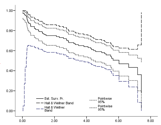
Figure 2.8 on page 35, as before we used chart editor to modify the plot including add reference lines
data list free
/subject time censor.
begin data
1  6 1
2 44 1
3 21 0
4 14 1
5 62 1
end data.

km time
/status =censor(1)
/percentile = (25 50 75)
/plot = survival.

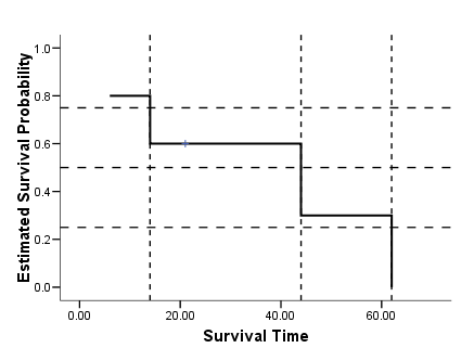
Table 2.5 on page 39 using the whas100 dataset. We can compute the confidence intervals manually based on the output in the percentiles table. For example, the calculation for computing the lower 95% confidence limit for 25% quantile should be (7.420 – 1.96*.176) = 7.07504. When we try to compute the upper 95% confidence limit, we get a number larger than the largest value of the time to event variable time in the data : 7.420 + 1.96*.176 = 7.76496 > 7.44 = max(time). In this case, as discussed in the book, it will be set to missing.
get file='C:Dataasa2whas100.sav'.
compute time = foltime/365.25.
km time
/status=folstatus(1)
/percentile = (25 50 75).


Table 2.6 on page 41 using the whas100 dataset.
get file='C:Dataasa2whas100.sav'.
compute time = foltime/365.25.

km time
/status=folstatus(1)
 /save survival(surv_km) se(surv_se).

compute var2_6 = surv_se**2/(surv_km**2*(ln(surv_km))**2).
compute z50 = abs(ln(-ln(surv_km)) - ln(-ln(.5)))/sqrt(var2_6).
compute cl  =ln(-ln(surv_km)) - 1.96*sqrt(var2_6).
compute cu  =ln(-ln(surv_km)) + 1.96*sqrt(var2_6).
compute l = exp(-exp(cu)).
compute u = exp(-exp(cl)).
exe.

use all.
compute filter_$=( ~ SYSMIS(surv_km)).
filter by filter_$.
exe.

sort cases by time (A).

list variables=time surv_km z50 l u
/cases =from 37.
    time    surv_km      z50        l        u

    4.10     .63000     2.45     .528     .716
    4.26     .62000     2.27     .517     .707
    4.32     .61000     2.09     .507     .698
    4.45     .60000     1.91     .497     .688
    4.57     .59000     1.73     .487     .679
    4.94     .58000     1.54     .477     .670
    5.13     .56885     1.33     .466     .659
    5.22     .55674     1.10     .453     .648
    5.51     .54037      .77     .435     .634
    5.56     .52348      .44     .416     .620
    5.65     .50479      .09     .396     .604
    6.03     .46873      .52     .347     .582
    6.63     .43267     1.04     .302     .556
    7.18     .36056     1.66     .200     .524
    7.42     .18028     2.08     .018     .482
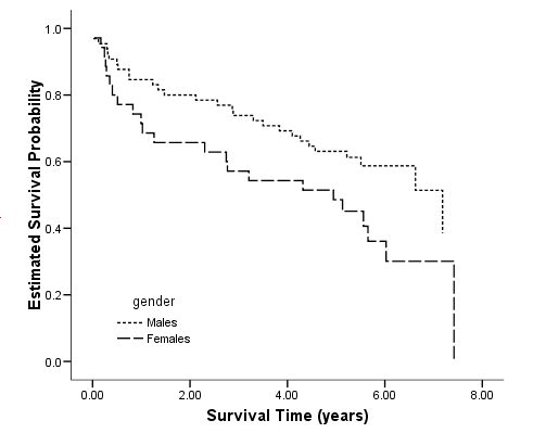
Figure 2.9 on page 46 using whas100 data.
get file='C:Dataasa2whas100.sav'.
compute time = foltime/365.25.

km time
/strata gender
/status=folstatus(1)
/save survival(surv_km).

graph
/scatterplot(bivar)=time with surv_km by gender.
Table 2.10 on page 50 using the small dataset shown in Table 2.9 on the same page to compute various quantities used in the tests for the equality of two survival functions.
data list free
/time d1 n1 d n.
begin data
  6    0  5  1  9
 14    1  5  1  8
 44    1  4  1  7
 98    1  2  2  4
104    1  1  1  2
114    0  0  1  1
end data.
compute e1 = n1*d/n.
compute v1 =n1*(n-n1)*d*(n-d)/(n**2*(n-1)).
recode v1 (sysmis= 0).
compute L = 1.
compute W = n.
compute T = sqrt(n).

if ($casenum = 1) P = (n+1-d)/(n+1).
if ($casenum>1) P =lag(P)*(n+1-d)/(n+1).
exe.
list.
 time d1    n1  d     n    e1    v1     L     W     T      P

    6  0     5  1     9   .56   .25  1.00  9.00  3.00     .90
   14  1     5  1     8   .63   .23  1.00  8.00  2.83     .80
   44  1     4  1     7   .57   .24  1.00  7.00  2.65     .70
   98  1     2  2     4  1.00   .33  1.00  4.00  2.00     .42
  104  1     1  1     2   .50   .25  1.00  2.00  1.41     .28
  114  0     0  1     1   .00   .00  1.00  1.00  1.00     .14
Table 2.11 on page 51 using the small data set above.
string testtype (A13).

*log-rank test.
compute q_n = L*(d1-e1).
compute q_d = L**2*v1.
descriptiive q_n q_d.

if ($casenum = 1) testtype = "Log-rank".
if ($casenum = 1) test= .1247**2*6/.2183.
exe.

*wilcoxon test.
compute q_n = W*(d1-e1).
compute q_d = W**2*v1.
descriptiive q_n q_d.

if ($casenum = 2) testtype = "Wilcoxon".
if ($casenum = 2) test= .3333**2*6/8.8889.
exe.
*Tarone-Ware test.
compute q_n = T*(d1-e1).
compute q_d = T**2*v1.
descriptiive q_n q_d.

if ($casenum = 3) testtype = "Tarone-Ware".
if ($casenum = 3) test= .2058**2*6/1.2741.
exe.
*Peto-Prentice test.
compute q_n = P*(d1-e1).
compute q_d = P**2*v1.
descriptiive q_n q_d.

if ($casenum = 4) testtype = "Peto-Prentice".
if ($casenum = 4) test= .0400**2*6/.0914.
exe.
compute p_value = 1-cdf.chisq(test, 1).
exe.

list
/variables = testtype test p_value.
testtype          test  p_value

Log-rank          .427     .513
Wilcoxon          .075     .784
Tarone-Ware       .199     .655
Peto-Prentice     .105     .746
Table 2.12 on page 51 using whas100 data. Note that SPSS 15 does not provide the Peto-Prentice test.
get file='C:Dataasa2whas100.sav'.
compute time = foltime/365.25.
km time  by gender
/status=folstatus(1)
/test logrank breslow tarone
/compare overall pooled.
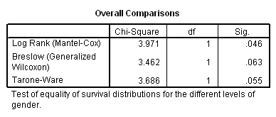
Table 2.13 on page 52 using whas100 data.
get file='C:Dataasa2whas100.sav'.
compute time = foltime/365.25.
recode age
  (0 thru 59=0)(60 thru 69=1)(70 thru 79=2)(80 thru 200=3)into agegroup .
exe.
km  time  by agegroup
/status=folstatus(1).
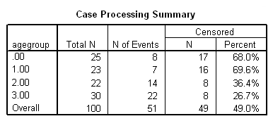

Figure 2.10 on page 55 using whas100 data and the agegroup variable generated in the previous example. The plot is heavily modified using the chart editor.
km  time  by agegroup
/status=folstatus(1)
/plot survival.
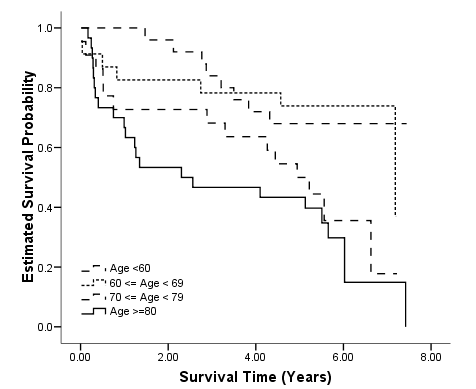
Table 2.15 on page 56. Note that SPSS 15 does not provide the Peto-Prentice test.
km time by agegroup
/status=folstatus(1)
/test logrank breslow tarone.
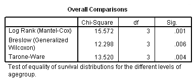
Table 2.16 on page 57, trend test. The vector of trend weights are set to be the midpoints of the four age groups. Note that SPSS 15 does not provide the Peto-Prentice test.
km time by agegroup
/status=folstatus(1)
/trend =(46, 65, 75, 86)
/test logrank breslow tarone
/compare overall pooled.
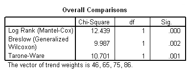
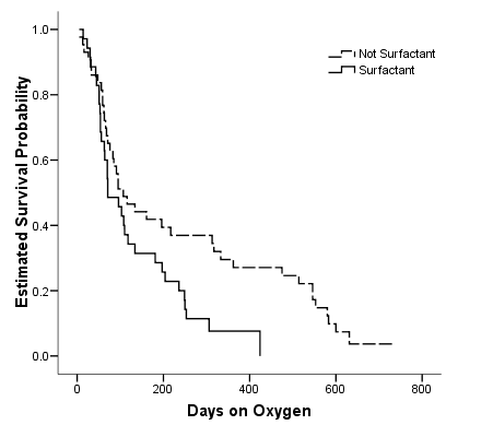
Figure 2.11 and Table 2.17 on page 58 using the bpd dataset.
get file ='C:Dataasa2bpd.sav'.
km ondays by surfact
/status=censor(1)
/plot survival
/test logrank breslow tarone
/compare overall pooled.
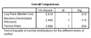
Figure 2.12, Figure 2.13 and Figure 2.14 are not doable in SPSS 16 since it does not produce Nelson-Aalen estimation.

