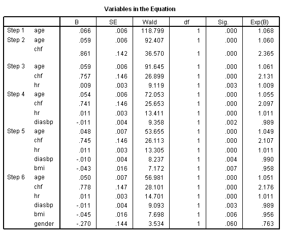
The whas500 data sets is used in this chapter.
Table 5.1 on page 142 using the whas500 data. Notice that SPSS does not provide Brookmeyer-Crowley confidence interval estimates for the medians. We will use the regular confidence interval estimates instead. To obtain the log-rank and partial likelihood ratio test, we used the coxreg procedure.
get file ='C:Dataasa2whas500.sav'.
compute time = lenfol /365.25.
exe.

* gender.
km time by gender
/status=fstat(1)
/print = mean.
coxreg time with gender
/status=fstat(1)
/categorical = gender.
* History of CVD.
km time by cvd
/status=fstat(1)
/print = mean.
coxreg time with cvd
/status=fstat(1)
/categorical = cvd.
* Atrial fibrillation.
km time by afb
/status=fstat(1)
/print = mean.
coxreg time with afb
/status=fstat(1)
/categorical = afb.
* Cardiogenic shock.
km time by sho
/status=fstat(1)
/print = mean.
coxreg time with sho
/status=fstat(1)
/categorical = sho.
* Congestive heart complications.
km time by chf
/status=fstat(1)
/print = mean.
coxreg time with chf
/status=fstat(1)
/categorical = chf.
* complete heart block.
km time by av3
/status=fstat(1)
/print = mean.
coxreg time with av3
/status=fstat(1)
/categorical = av3.
* MI order.
km time by miord
/status=fstat(1)
/print = mean.
coxreg time with miord
/status=fstat(1)
/categorical = miord.
* MI type.
km time by mitype
/status=fstat(1)
/print = mean.
coxreg time with mitype
/status=fstat(1)
/categorical = mitype.
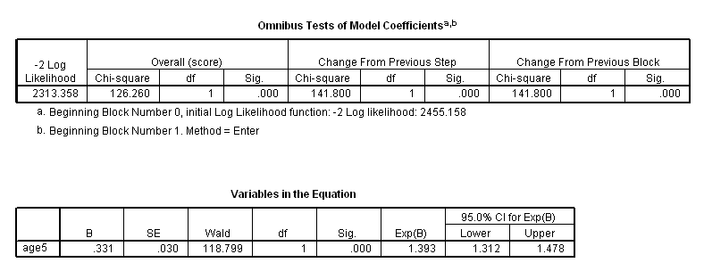
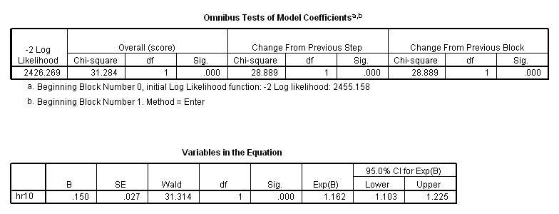
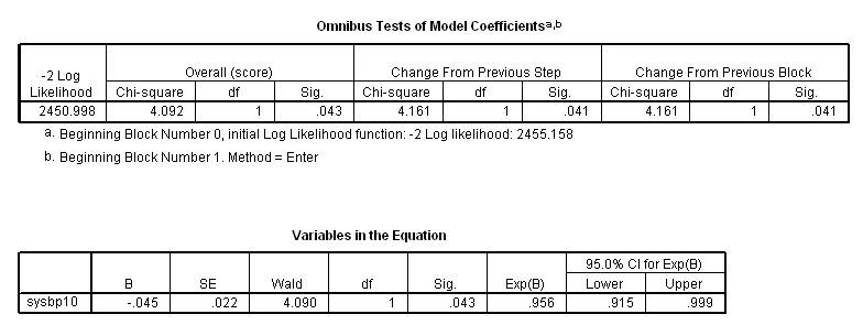
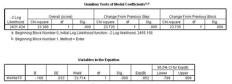
Table 5.2 on page 143 using the whas500 data, moving on to continuous variables.
* 5 years change in age.
compute age5 = age/5.
exe.
coxreg time with age5
/status=fstat(1)
/print = ci.
* 10 beats change in heart rate.
compute hr10 = hr/10.
exe.
coxreg time with hr10
/status=fstat(1)
/print = ci.
* 10 mmHg change in systolic blood pressure.
compute sysbp10 = sysbp/10.
exe.
coxreg time with sysbp10
/status=fstat(1)
/print = ci.
* 10 mmHg change in diastolic blood pressure.
compute diasbp10 = diasbp/10.
exe.
coxreg time with diasbp10
/status=fstat(1)
/print = ci.
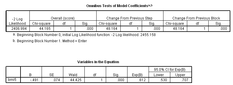
* 5 unit change in body mass index.
compute bmi5 = bmi/5.
exe.
coxreg time with bmi5
/status=fstat(1)
/print = ci.
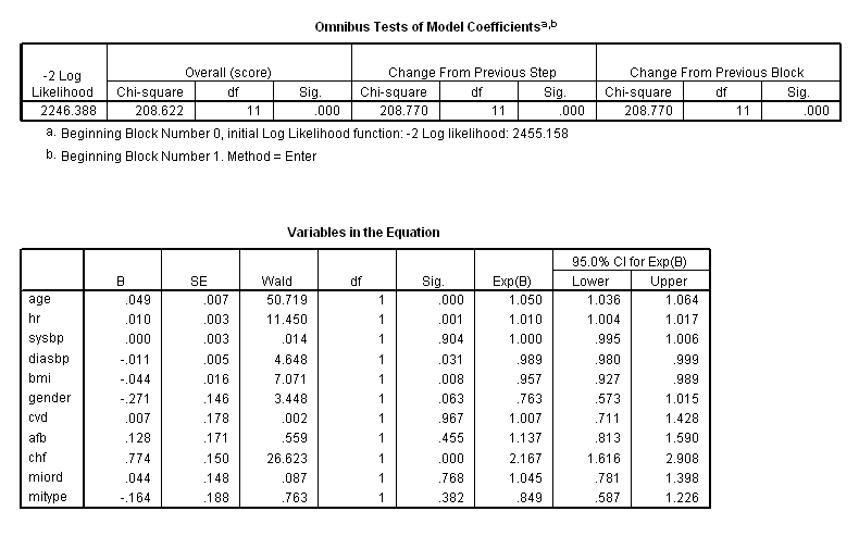
Table 5.3, Table 5.4, Table 5.5 and Table 5.6 on pages 143-145 using the whas500 data in a multivariate model.
* Table 5_3.
coxreg time with age hr sysbp diasbp bmi gender cvd afb chf miord mitype
/status=fstat(1)
/print = ci.
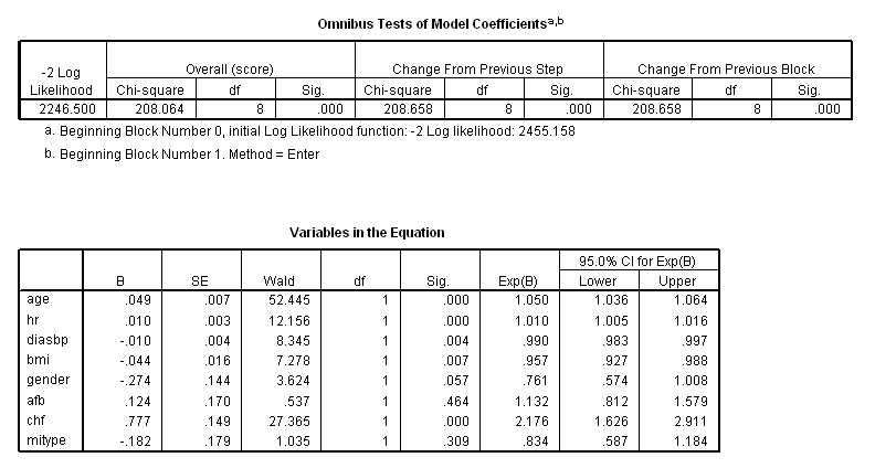
* Table 5_4.
coxreg time with age hr diasbp bmi gender afb chf miord mitype
/status=fstat(1)
/print = ci.
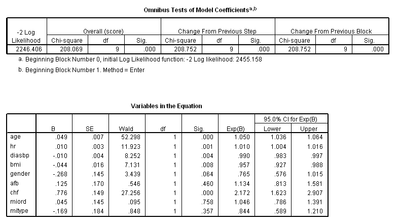
* Table 5_5.
coxreg time with age hr diasbp bmi gender afb chf mitype
/status=fstat(1)
/print = ci.
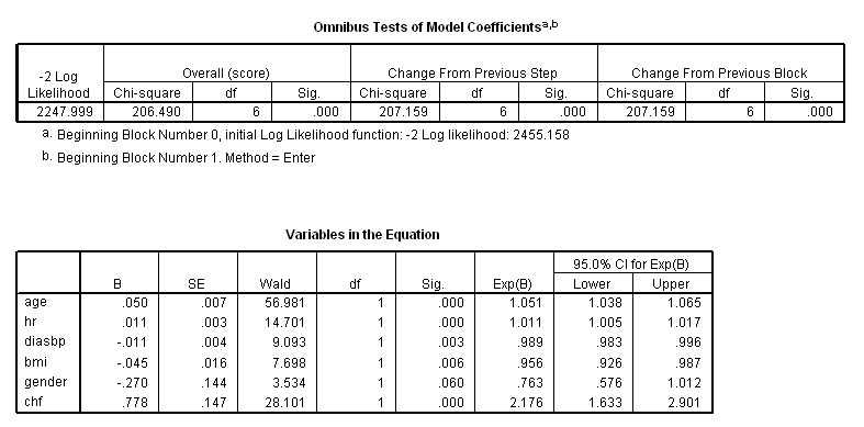
* Table 5_6.
coxreg time with age hr diasbp bmi gender chf
/status=fstat(1)
/print = ci.
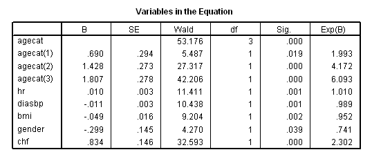
Table 5.7 on page 146 continuing to use the whas500 data.
rank variables =age  (A)
/ntiles (4) into agecat
/ties=low.

coxreg time with agecat hr diasbp bmi gender chf
/status=fstat(1)
/categorical = agecat
/contrast(agecat) = indicator(1).
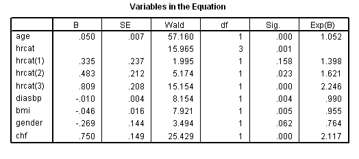
rank variables =hr  (A)
/ntiles (4) into  hrcat
/ties=low.

coxreg time with age hrcat diasbp bmi gender chf
/status=fstat(1)
/categorical = hrcat
/contrast(hrcat) = indicator(1).
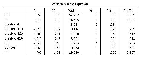
rank variables = diasbp (A)
 /ntiles (4) into diasbpcat
  /ties=low.

coxreg time with age hr diasbpcat bmi gender chf
/status=fstat(1)
/categorical = diasbpcat
/contrast(diasbpcat) = indicator(1).
rank variables = bmi (A)
 /ntiles (4) into bmicat
  /ties=low.

coxreg time with age hr diasbp bmicat gender chf
/status=fstat(1)
/categorical = bmicat
/contrast(bmicat) = indicator(1).
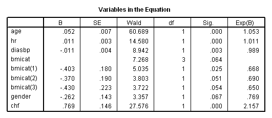
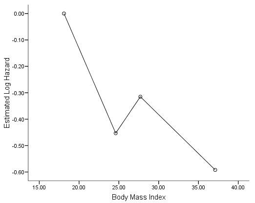
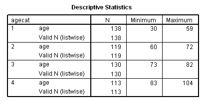
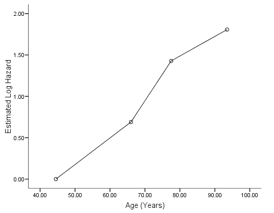
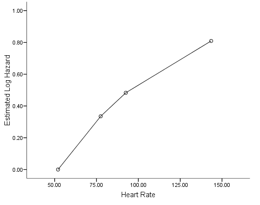
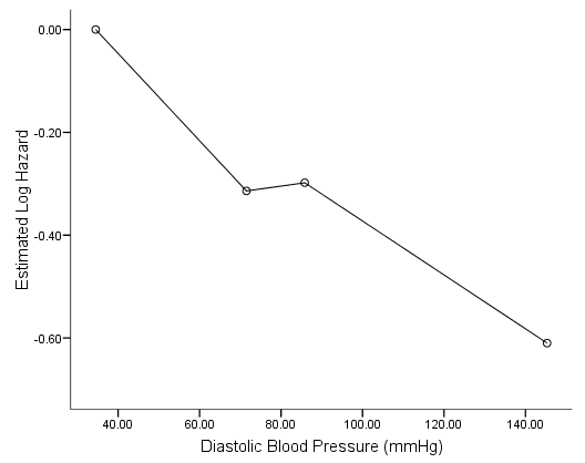
Figure 5.1 on page 146 based on the results from previous Table 5.7. The definition of the quartile midpoints is the average of minimal and maximal value within each quartile.
sort cases by agecat.
split file
layered by agecat.

descriptives variables = age
/statistics = min max.
* Age.
data list free
/age coeff.
begin data
44.5   0
66   .690
77.5 1.428
93.5 1.807
end data.
graph  /scatterplot(bivar) =age with coeff.
* Heart Rate.
data list free
/hr coeff.
begin data
52   0
77.5   .335
92.5 .483
143.5 .809
end data.
graph  /scatterplot(bivar) =hr with coeff.
data list free
* Diastolic Blood Pressure.
/diasbp coeff.
begin data
34.5   0
71.5  -.314
85.8 -.298
145.3 -.610
end data.
graph  /scatterplot(bivar) =diasbp with coeff.
* Body Mass Index.
data list free
/bmi coeff.
begin data
18.1   0
24.6  -.453
27.7 -.315
37.1 -.592
end data.
graph  /scatterplot(bivar) =bmi with coeff.
Table 5.8 on page 147 using the whas500 data. Because that SPSS does not provide a routine for fractional polynomial regression, we will simply reproduce the table using the transformations discussed in the section.
get file ='C:whas500.sav'.
compute time = lenfol /365.25.
exe.
* Model 1: bmi not in the model.
coxreg time with age hr diasbp gender chf
/status=fstat(1).
* Model 2: bmi in the model as a linear term.
coxreg time with age hr diasbp gender chf bmi
/status=fstat(1).
* Model 3: bmi in the model as bmi^(-2).
compute bmi2 = bmi**(-2).
coxreg time with age hr diasbp gender chf bmi2
/status=fstat(1).
* Model 4: bmi in the model as bmi^2 and bmi^3.
compute bmi_sq = bmi**2.
compute bmi_cu = bmi**3.
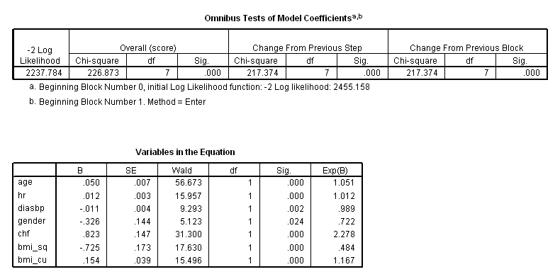
coxreg time with age hr diasbp gender chf bmi_sq bmi_cu
/status=fstat(1).
Table 5.8 based on the four models above. A few words about the determination of the degrees of freedom in the Table shown below. The degrees of freedom in the table is the extra degrees of freedom related to the variable of bmi that we have tried to find the best transformation for. So when it is not in the model, there is no degrees of freedom associated with it, therefore it is zero. A linear term will add 1 degree of freedom. The third model is based on the "best" model with one single term of transformation of the variable bmi. The determination of the best transformation (in this case, it is power of -2) takes a degree of freedom. Therefore, together with the parameter estimate, it takes two degrees of freedom. For the case of two terms, we will have two parameters for the best transformation and two regression coefficients to be estimated. It thus yields four degrees of freedom.
data list free /ll df.
begin data.
2255.945 0
2247.999 1
2241.668 2
2237.784 4
end data.
if $casenum>1 gstat = 2247.999 -ll.
compute chisq = lag(ll) - ll.
compute difdf = df -lag(df).
compute pvalue = 1- cdf.chisq(chisq,difdf).
exe.
list variables = ll gstat pvalue.
     ll    gstat   pvalue

 2255.95      .      .
 2248.00      .00    .0048
 2241.67     6.33    .0119
 2237.78    10.21    .1434
Figure 5.2a on page 149 using model without bmi on the whas500 data. The only place in SPSS that is related to local linear regression is via the Chart Editor. Shown below, we chose Loess fit method with %80 of points to fit and triweight kernel.
get file ='C:Dataasa2whas500.sav'.
compute time = lenfol /365.25.
exe.
coxreg time with age hr diasbp gender chf
/status=fstat(1)
/save hazard(Hazard).

compute mgale = fstat - Hazard.
exe.
graph /scatterplot(bivar) = bmi with mgale.
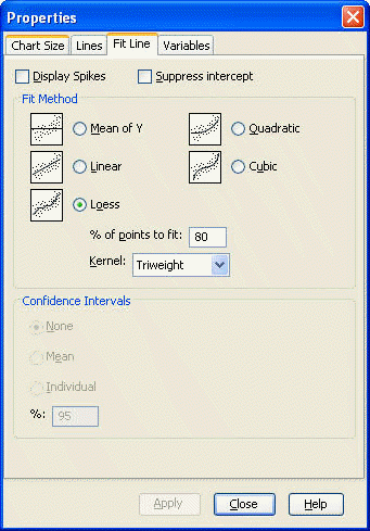
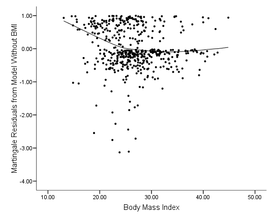
Figure 5.2b and Figure 5.3 on page 149 and 150. Unfortunately, SPSS (up to version 16) does not allow us to saving the predicted values based on the Loess fit. That means we will not be able to produce figure 5.2b and Figure 5.3.
Table 5.9 on page 150 using the whas500 data.
get file ='C:Dataasa2whas500.sav'.
compute time = lenfol /365.25.
compute bmi_sq = (bmi/10)**2.
compute bmi_cu = (bmi/10)**3.
coxreg time with age hr diasbp gender chf bmi_sq bmi_cu
/status=fstat(1).
Table 5.10 on page 151 using the whas500 data.
* Model 1: Interaction of age and bmi variables.
coxreg time
/method = enter age hr diasbp gender chf bmi_sq bmi_cu
/method = enter age*bmi_sq age*bmi_cu
/status=fstat(1).

* Model 2: Interaction of age with hr.
coxreg time
/method = enter age hr diasbp gender chf bmi_sq bmi_cu
/method = enter age*hr
/status=fstat(1).
* Model 3: Interaction of age with diasbp.
coxreg time
/method = enter age hr diasbp gender chf bmi_sq bmi_cu
/method = enter age*diasbp
/status=fstat(1).
* Model 4: Interaction of age with gender.
coxreg time
/method = enter age hr diasbp gender chf bmi_sq bmi_cu
/method = enter age*gender
/status=fstat(1).
* Model 5: Interaction of age with chf.
coxreg time
/method = enter age hr diasbp gender chf bmi_sq bmi_cu
/method = enter age*chf
/status=fstat(1).
* Model 6: Interaction of gender with bmi variables.
coxreg time
/method = enter age hr diasbp gender chf bmi_sq bmi_cu
/method = enter gender*bmi_sq gender*bmi_cu
/status=fstat(1).
* Model 7: Interaction of gender with hr.
coxreg time
/method = enter age hr diasbp gender chf bmi_sq bmi_cu
/method = enter gender*hr
/status=fstat(1).

* Model 8: Interaction of gender with diasbp.
coxreg time
/method = enter age hr diasbp gender chf bmi_sq bmi_cu
/method = enter gender*diasbp
/status=fstat(1).

* Model 9: Interaction of gender with chf.
coxreg time
/method = enter age hr diasbp gender chf bmi_sq bmi_cu
/method = enter gender*chf
/status=fstat(1).

Table 5.11 and Table 5.12 on page 152 using the whas500 data.
coxreg time
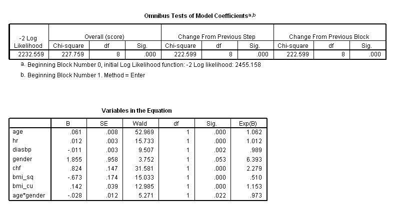
/method = enter age hr diasbp gender chf bmi_sq bmi_cu age*gender
/status=fstat(1).
coxreg time
/method = enter age hr diasbp gender chf bmi_sq bmi_cu
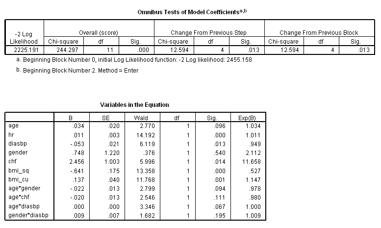
/method = enter age*gender age*chf age*diasbp gender*diasbp
/status=fstat(1).
Table 5.13 on page 153 is Table 5.11 shown in previous example.
Table 5.14 on page 158 using whas500 data.
get file ='C:Dataasa2whas500.sav'.
compute time = lenfol /365.25.
exe.

coxreg time
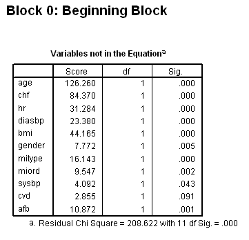
/method = fstep  age chf hr diasbp bmi gender mitype miord sysbp cvd afb
/criteria = pin(.25)
/status=fstat(1).
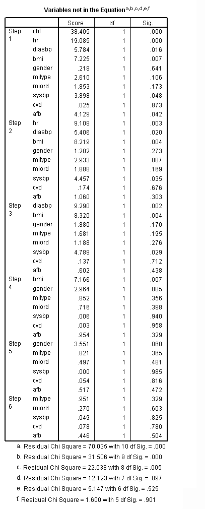
Table 5.15 on page 161. SPSS does not have stepwise with method="BEST" approach as to version 16.
Table 5.16 on page 165. SPSS does not have a procedure for fractional polynomial regression as to version 16.


