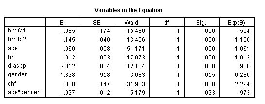
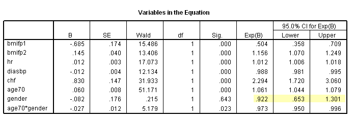
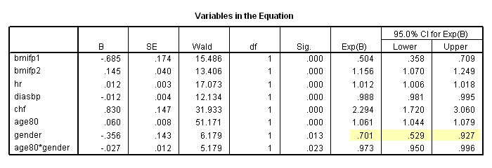
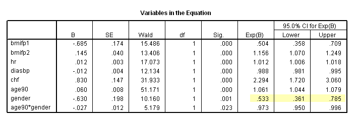
The whas500 data set is used in this chapter.
Table 6.1 on page 180. SPSS (as of version 16) does not offer score test for proportionality hazards.
Figure 6.1 on page 181, Figure 6.2 on page 182 and Figure 6.3 on page 183 using whas500 data. To add the loess smoothing, we selected tri-cube kernel smooth with %80 percent of data points used at each point in the SPSS chart editor.
get file ='C:Dataasa2whas500.sav'.
compute time = lenfol /365.25.
compute bmifp1 = (bmi/10)**2.
compute bmifp2 = (bmi/10)**3.
exe.

oms
/select tables
/if subtypes = ['Correlation Matrix of Regression Coefficients']
/destination format = sav
outfile  = 'c:dataasa2corr.sav'.
oms
/select tables
/if subtypes =  ['Variables in the Equation']
/destination format = sav
outfile  = 'c:dataasa2parms.sav'.
coxreg time
/method = enter bmifp1 bmifp2 age hr diasbp gender chf age*gender
/status fstat(1)
/print = corr
/save presid (ssr).
omsend.
km time
/status=fstat(1)
/save survival(survival).

compute logtime = ln(time).
exe.

use all.
filter by fstat.
exe.
matrix.
/*main part of this matrix program is  for creating the covariance matrix*/
get corr /file="c:dataasa2corr.sav"
 /variables=bmifp1 bmifp2 age hr diasbp gender chf
/missing = 0.

compute d=nrow(corr).
compute a = make(d+1, d+1, 0).
loop i = 1 to d.
   loop j = i+1 to d+1.
     compute a(i, j) = corr(j-1, i).
     compute a(j,i) =corr(j-1, i).
   end loop.
end loop.
compute c = ident(d+1) + a.

get se /file="c:dataasa2parms.sav"
/variables = se.
compute sigma=mdiag(se).
compute cov = sigma*c*sigma.
get res
  /variables  = ssr1 to ssr8
  /file=* .
compute total = nrow(res).
compute sres = total*res*cov.
get others
/variables = time survival logtime
/file=*.
save {others, sres}
/outfile = "c:dataasa2scaled_schoenfeld.sav"
/variables = time survival logtime sr_bmi1 sr_bmi2 sr_age sr_hr sr_diasbp sr_gender sr_chf sr_axg.
end matrix.
get file ='C:Dataasa2scaled_schoenfeld.sav'.
rank varaibles = time (A) /rank into Rtime /print = no /ties= mean. * figure 6.1a. graph /scatterplot(bivar) = logtime with sr_hr.* figure 6.1b. graph /scatterplot(bivar) = time with sr_hr.
* figure 6.1c. graph /scatterplot(bivar) = survival with sr_hr.
* figure 6.1d. graph /scatterplot(bivar) = Rtime with sr_hr.
* figure 6.2a. graph /scatterplot(bivar) = logtime with sr_chf.
* figure 6.2b. graph /scatterplot(bivar) = time with sr_chf.
* figure 6.2c. graph /scatterplot(bivar) = survival with sr_chf.
* figure 6.2d. graph /scatterplot(bivar) = Rtime with sr_chf.
* figure 6.3a. graph /scatterplot(bivar) = logtime with sr_age.
* figure 6.3b. graph /scatterplot(bivar) = time with sr_age.
* figure 6.3c. graph /scatterplot(bivar) = survival with sr_age.
* figure 6.3d. graph /scatterplot(bivar) = Rtime with sr_age.
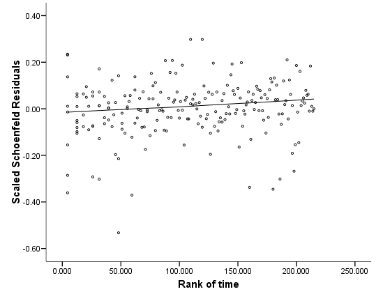
Figure 6.4 and Figure 6.5 on page 186 using the whas500 data. SPSS (up to version 16) does not provide score residuals.
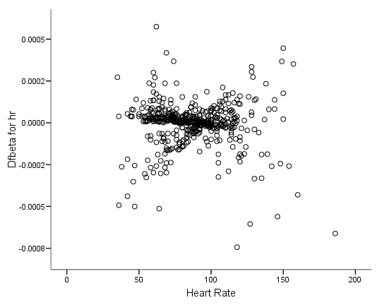
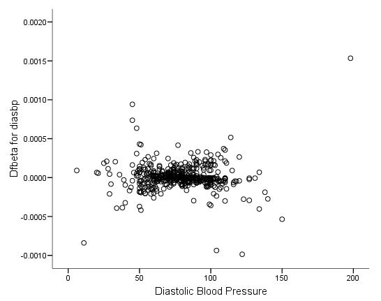
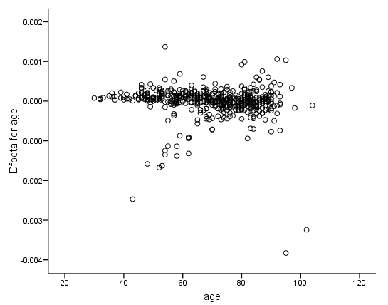
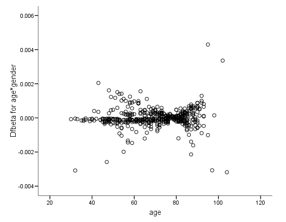
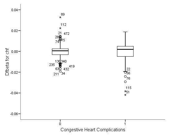
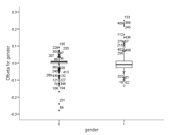
Figure 6.6 on page 187 and Figure 6.7 on page 188 using whas500 data. The estimate of DFBETA is based the augmented regression model described by Storer and Crowley in their article A diagnostic for Cox regression and general conditional likelihoods appeared in the Journal of the American Statistical Association, Vol. 80, 1985. This definition of DFBETA is different but closely related to the definition of DFBETA as scaled score residuals used in the book. In practice, the two forms are not far apart.
get file ='C:Dataasa2whas500.sav'. compute time = lenfol /365.25. compute bmifp1 = (bmi/10)**2. compute bmifp2 = (bmi/10)**3. exe. coxreg time /method = enter bmifp1 bmifp2 age hr diasbp gender chf age*gender /status fstat(1) /print = corr /save dfbeta (dfbeta). * figure 6.6a. compute dfbeta1 = -dfbeta1. graph /scatterplot(bivar) = bmi with dfbeta1.* figure 6.6b. compute dfbeta2 = -dfbeta2. graph /scatterplot(bivar) = bmi with dfbeta2.
* figure 6.6c.
compute dfbeta4 = -dfbeta4.
graph /scatterplot(bivar) = hr with dfbeta4.
* figure 6.6d.
compute dfbeta5 = -dfbeta5.
graph /scatterplot(bivar) = diasbp with dfbeta5.
*figure 6.7a.
compute dfbeta3 = -dfbeta3.
graph /scatterplot(bivar) = age with dfbeta3.
*figure 6.7b.
compute dfbeta8 = -dfbeta8.
graph /scatterplot(bivar) = age with dfbeta8.
*figure 6.7c.
compute dfbeta7 = -dfbeta7.
examine variables = dfbeta7 by chf
/plot=boxplot
/statistics = none
/nototal.
*figure 6.7d.
compute dfbeta6 = -dfbeta6.
examine variables = dfbeta6 by gender
/plot=boxplot
/statistics = none
/nototal.
Table 6.2 on page 189 using the whas500 data. As mentioned before, the definition of DFBETA in SPSS is different from the book, although in practice both are defined as the influence of an observation on parameter estimates. We used the SPSS definition of DFBETA and defined the likelihood displacement based on it and the variance-covariance matrix of the parameter estimates.
Most of the code below is for getting the variance-covariance matrix from the correlation matrix. We first identify points with high-leverage, high-influential or large Cook’s Distance based on the plots created in previous example and then list them together.
get file ='C:Dataasa2whas500.sav'.
compute time = lenfol /365.25.
compute bmifp1 = (bmi/10)**2.
compute bmifp2 = (bmi/10)**3.
exe.

oms
/select tables
/if
   subtypes = ['Correlation Matrix of Regression Coefficients']
/destination format = sav
outfile  = 'c:dataasa2corr.sav'.
oms
/select tables
/if
   subtypes =  ['Variables in the Equation']
/destination format = sav
outfile  = 'c:dataasa2parms.sav'.
coxreg time
/method = enter bmifp1 bmifp2 age hr diasbp gender chf age*gender
/status fstat(1)
/print = corr
/save = Hazard(Haz) dfbeta(dfbeta).
omsend.

compute mart =  fstat - Haz.
exe.

set mxloop=500.
matrix.
get corr /file="c:dataasa2corr.sav"
 /variables=bmifp1 bmifp2 age hr diasbp gender chf
/missing = 0.

compute d=nrow(corr).
compute a = make(d+1, d+1, 0).
loop i = 1 to d.
   loop j = i+1 to d+1.
     compute a(i, j) = corr(j-1, i).
     compute a(j,i) =corr(j-1, i).
   end loop.
end loop.
compute c = ident(d+1) + a.

get se /file="c:dataasa2parms.sav"
/variables = se.
compute sigma=mdiag(se).
compute cov = sigma*c*sigma.

get dfbeta
  /variables  = dfbeta1 to dfbeta8
  /file=* .

compute ld = make(500,1, 0).
   loop i = 1 to 500.
     compute ld(i) = dfbeta(i, :)*inv(cov)*t(dfbeta(i, :)).
   end loop.

get others
/variables = id bmi age hr diasbp gender chf  mart
/missing = -9999
/file=*.

save {others, dfbeta, ld}
/outfile = "c:dataasa2ld.sav"
/variables =id bmi age hr diasbp gender chf mart dfbeta1 dfbeta2
            dfbeta3 dfbeta4 dfbeta5 dfbeta6 dfbeta7 dfbeta8 ld.
end matrix.

get file ='c:dataasa2ld.sav'.
use all.
compute  filter =(dfbeta1<-.05 & bmi <20).
filter by filter.
exe.
list variables = id bmi dfbeta1.
     id      bmi  dfbeta1

   89.00    15.93     -.11
  112.00    14.84     -.07
  115.00    18.90     -.06
use all.
compute  filter =(dfbeta2> 0.01 & bmi <20 | dfbeta2 <-.01 & bmi>41).
filter by filter.
exe.
list variables = id bmi dfbeta2.
      id      bmi  dfbeta2

   89.00    15.93      .02
  112.00    14.84      .01
  115.00    18.90      .01
  256.00    44.84     -.01
compute  filter =(hr >170).
filter by filter.
exe.
list variables = id hr dfbeta4.
      id       hr  dfbeta4

  472.00   186.00      .00
use all.
compute  filter =(diasbp >190).
filter by filter.
exe.
list variables = id diasbp dfbeta5.
      id   diasbp  dfbeta5

  416.00   198.00      .00
use all.
compute  filter =(age > 85 & dfbeta3 >.002).
filter by filter.
exe.
list variables = id age dfbeta3.
      id      age  dfbeta3

   89.00    95.00      .00
  251.00   102.00      .00
use all.
compute  filter =(age <40 & dfbeta8 >.002 | age >70 & dfbeta8 <-.002).
filter by filter.
exe.
list variables = id age dfbeta8.
      id      age  dfbeta8

   89.00    95.00      .00
  153.00    32.00      .00
  251.00   102.00      .00
use all.
compute  filter =(chf = 1 & dfbeta7 >.03).
filter by filter.
exe.
list variables = id chf dfbeta7.
      id      chf  dfbeta7

   51.00     1.00      .04
  115.00     1.00      .04
use all.
compute  filter =(gender = 0 & dfbeta6 >.15).
filter by filter.
exe.
list variables = id gender dfbeta6.
      id   gender  dfbeta6

   89.00      .00      .28
  194.00      .00      .17
  251.00      .00      .24
use all.
compute  filter =(mart<-3 & ld >.2).
filter by filter.
exe.
list variables = id bmi age hr diasbp gender chf.
      id      bmi      age       hr   diasbp   gender      chf

   89.00    15.93    95.00    62.00    45.00      .00      .00
  115.00    18.90    81.00   118.00    70.00     1.00     1.00
use all.
compute  filter =(id = 51 | id = 89 | id = 112 | id = 115 | id = 153 |
                  id = 194 | id = 251 | id = 256 | id = 416 | id = 472).
filter by filter.
exe.
list variables = id bmi age hr diasbp gender chf.
      id      bmi      age       hr   diasbp   gender      chf

   51.00    22.45    80.00   105.00    72.00      .00     1.00
   89.00    15.93    95.00    62.00    45.00      .00      .00
  112.00    14.84    87.00   105.00   104.00     1.00      .00
  115.00    18.90    81.00   118.00    70.00     1.00     1.00
  153.00    39.94    32.00   102.00    83.00     1.00      .00
  194.00    24.21    43.00    47.00    90.00      .00     1.00
  251.00    22.27   102.00    89.00    60.00      .00     1.00
  256.00    44.84    53.00    96.00    99.00     1.00      .00
  416.00    28.55    80.00    64.00   198.00      .00      .00
  472.00    25.40    72.00   186.00    84.00      .00      .00
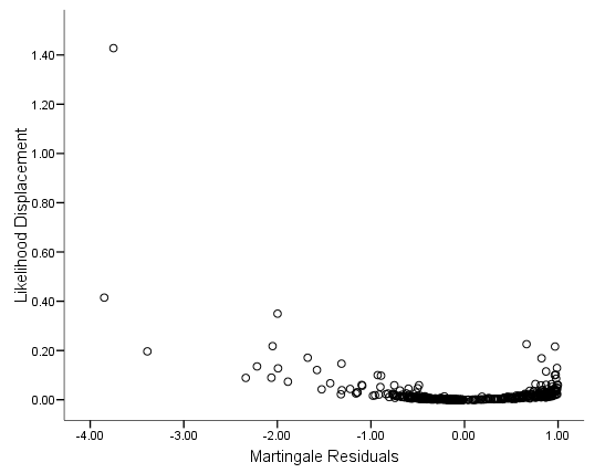
Figure 6.8 on page 190 using the Martingale residuals calculated on the whas500 data.
graph /scatterplot(bivar) = mart with ld.
Table 6.3 on page 191 using the whas500 data.
get file ='C:Dataasa2whas500.sav'.
compute time = lenfol /365.25.
compute bmifp1 = (bmi/10)**2.
compute bmifp2 = (bmi/10)**3.
exe.

use all.
compute filter = ( diasbp ~= 198).
filter by filter.
exe.
coxreg time
/method = enter bmifp1 bmifp2 age hr diasbp gender chf age*gender
/status fstat(1).
Table 6.4 on page 194 using the whas500 data. Notice that since the linear prediction in SPSS is mean-adjusted, the cut points in the table produced below are also mean-adjusted. Our quantiles do not exactly match those in the text.
get file ='C:Dataasa2whas500.sav'.
compute time = lenfol /365.25.
compute bmifp1 = (bmi/10)**2.
compute bmifp2 = (bmi/10)**3.
exe.

use all.
compute filter = ( diasbp ~= 198).
filter by filter.
exe.
coxreg time
/method = enter bmifp1 bmifp2 age hr diasbp gender chf age*gender
/status fstat(1)
/save =Hazard(Haz)  xbeta(xb) .

rank variable = xb
/ntiles(5) into quintile.

compute one = 1.
exe.
aggregate
/outfile = "c:dataasa2table64.sav"
/break = quintile
/cut_point = max(xb)
/observed = sum(fstat)
/expected = sum(Haz)
/count =sum(one).


get file = "c:dataasa2table64.sav".
 compute z = abs((observed-expected)/sqrt(expected)).
compute p = 2*(1-cdf.normal(z, 0, 1)).
list variables = quintile cut_point count observed expected z p.
quintile cut_point count observed expected z p
     1    -1.10338    99.00     6.00     8.03      .72      .47
     2     -.29737   101.00    15.00    20.89     1.29      .20
     3      .33435    99.00    40.00    38.11      .31      .76
     4     1.04312   100.00    66.00    54.00     1.63      .10
     5     3.19637   100.00    87.00    93.23      .65      .52
Table 6.5 on page 196 is the same as Table 6.3 on page 191 using the whas500 data.
Table 6.6 on page 197 and Table 6.7 on page 198 based on the whas500 model presented in Table 6.5.
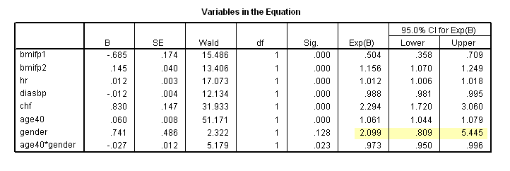
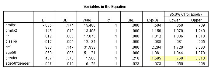
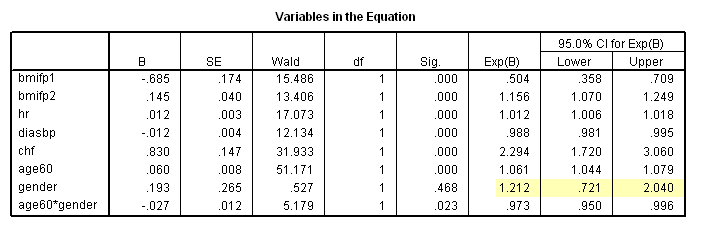
Table 6.7 can be done in at least two different but equivalent ways. One way is to use calculate the hazard ratio for different age group using the same model given by Table 6.5 and the variance-covariance matrix of the parameter estimates. Another way is to center the age variable and rerun the model. The effect of gender can then be read off directly from the table of coefficients. We will present the latter method since it is less straightforward in SPSS to obtain the variance-covariance matrix. Also notice, the difference presented here is solely due to rounding error.
get file ='C:Dataasa2whas500.sav'.
compute time = lenfol /365.25.
compute bmifp1 = (bmi/10)**2.
compute bmifp2 = (bmi/10)**3.
exe.

use all.
compute filter = ( diasbp ~= 198).
filter by filter.
exe.
compute hr10 = hr/10.
compute diasbp10 = diasbp/10.
exe.

* Table 6.6.
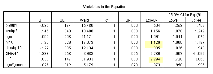
coxreg time
/method = enter bmifp1 bmifp2 age hr10 diasbp10 gender chf age*gender
/status fstat(1)
/print =ci.
* Table 6.7, age = 40.
compute age40 = age-40.
exe.
coxreg time
/method = enter bmifp1 bmifp2 hr diasbp chf age40 gender age40*gender
/status fstat(1)
/print =ci.
* Table 6.7, age = 50.
compute age50 = age-50.
exe.
coxreg time
/method = enter bmifp1 bmifp2 hr diasbp chf age50 gender age50*gender
/status fstat(1)
/print =ci.
* Table 6.7, age = 60.
compute age60 = age-60.
exe.
coxreg time
/method = enter bmifp1 bmifp2 hr diasbp chf age60 gender age60*gender
/status fstat(1)
/print =ci.
* Table 6.7, age = 70.
compute age70 = age-70.
exe.
coxreg time
/method = enter bmifp1 bmifp2 hr diasbp chf age70 gender age70*gender
/status fstat(1)
/print =ci.
* Table 6.7, age = 80.
compute age80 = age-80.
exe.
coxreg time
/method = enter bmifp1 bmifp2 hr diasbp chf age80 gender age80*gender
/status fstat(1)
/print =ci.
* Table 6.7, age = 90.
compute age90 = age-90.
exe.
coxreg time
/method = enter bmifp1 bmifp2 hr diasbp chf age90 gender age90*gender
/status fstat(1)
/print =ci.
Figure 6.9 on page 202 using the same model appeared in Table 6.3.
get file ='C:Dataasa2whas500.sav'.
compute time = lenfol /365.25.
compute bmifp1 = (bmi/10)**2.
compute bmifp2 = (bmi/10)**3.
exe.

use all.
select if (idasbp ~=198).
exe.
coxreg time
/method = enter bmifp1 bmifp2 age hr diasbp gender chf age*gender
/status fstat(1)
/print =corr.

compute a = bmifp1 - 9.9225.
compute b = bmifp2 - 31.25588.

compute ln_hr = (-0.685)*a+.145*b.
compute hr = exp(ln_hr).
exe.

* variance for bmifp1 is .174**2.
* variance for bmifp2 is .040**2.
* the covariance is corr*se_a*se_b.

compute se_ln_hr = sqrt((a**2)*(.174**2)+b**2*(.040**2)+2*a*b*(-.989)*.174*.040).
compute hr_l  = exp(ln_hr -1.96*se_ln_hr).
compute hr_u = exp(ln_hr+1.96*se_ln_hr).
exe.

use all.
compute filter = ( hr_u <10).
filter by filter.
exe.

graph
/scatterplot(overlay)=bmi bmi bmi with hr hr_u hr_l (pair).
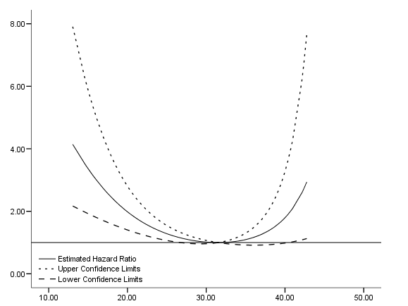
Table 6.8 on page 203 using the previous model. We first create a data set with values of bmi ranging from 15 to 40. Then we compute the predicted hazard ratio based on the model using the approach outlined on page 201. The discrepancy of the table below from the table in the book is due to rounding error.
new file.
input program.
loop i = 1 to 6.
compute bmi = 15 + (i -1)*5.
end case.
end loop.
end file.
end input program.
exe.
compute bmifp1 = (bmi/10)**2.
compute bmifp2 = (bmi/10)**3.
compute a = bmifp1 - (31.5/10)**2.
compute b = bmifp2 - (31.5/10)**3.

compute ln_hr = (-0.685)*a+.145*b.
compute hr = exp(ln_hr).
exe.
* variance for bmifp1 is .174**2.
* variance for bmifp2 is .040**2.

* the covariance is corr*se_a*se_b.

compute se_ln_hr = sqrt((a**2)*(.174**2)+b**2*(.040**2)+2*a*b*(-.989)*.174*.040).
compute hr_l  = exp(ln_hr -1.96*se_ln_hr).
compute hr_u = exp(ln_hr+1.96*se_ln_hr).
exe.

list variables = bmi hr hr_l hr_u.
     bmi       hr     hr_l     hr_u

   15.00     3.36     1.92     5.88
   20.00     1.98     1.40     2.80
   25.00     1.28     1.07     1.54
   30.00     1.01      .96     1.07
   35.00     1.09      .92     1.30
   40.00     1.79      .98     3.27
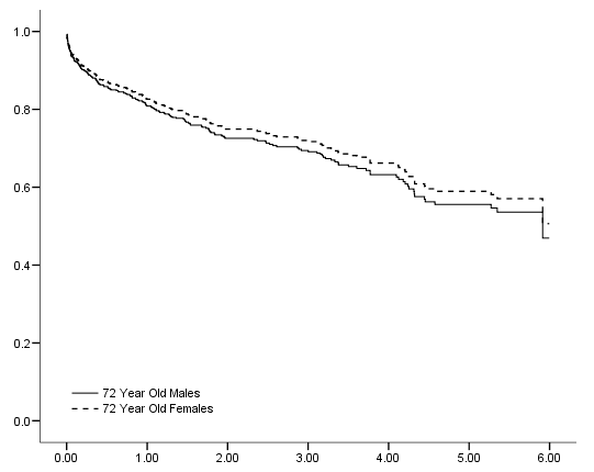
Figure 6.9 on page 204 using the same model as in the previous example. First we save the cumulative hazard function and the xbeta score which will be used to calculate the baseline score when all the variables are set to zero. XBETA in SPSS is the linear combination of mean corrected covariates times regression coefficients from the model. Therefore, the relationship between the cumulative hazard function and the xbeta score is:
H(t)/exp(xbeta) = H0(t)*exp(the linear combination of mean values of covariates times regression coefficients)
get file ='C:Dataasa2whas500.sav'.
compute time = lenfol /365.25.
compute bmifp1 = (bmi/10)**2.
compute bmifp2 = (bmi/10)**3.
exe.

use all.
compute filter = ( diasbp ~= 198).
filter by filter.
exe.

coxreg time
/method = enter bmifp1 bmifp2 age hr diasbp gender chf age*gender
/status fstat(1)
/print = baseline
/save = xbeta(xb) Hazard(haz).

*notice that xb is mean-adjusted already.
compute mean_xb = 7.373*(-.685) + 21.258*(.145) + 69.826*(.06) + 87.064*(.012)
                  + 78.026*(-.012) + .401*(1.838) + .311*.830 + 29.948*(-.027).

compute base_haz = haz/exp(xb)/exp(mean_xb).
compute base_surv = exp(-base_haz).
compute r = xb + bmifp1*(-.685) + bmifp2*(.145) + hr*(.012) + diasbp*(-.011) + chf*(.824).

examine variables = r
/plot none
/percentiles(50).
compute s_male =   base_surv**(exp(-1.79+.06*72)).
compute s_female = base_surv**(exp(-1.79+.06*72 + 1.838 - .027*72)).
exe.

use all.
compute filter = ( diasbp ~= 198 & time<6).
filter by filter.
exe.

graph /scatterplot(overlay) =time time with s_male s_female (pair).
