Page 447 Table 17.1
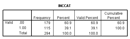
get file 'c:cama4depress.sav'.

compute inccat = 0.
if income ge 20 inccat = 1.
crosstabs sex by inccat.
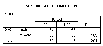
Page 448 Table 17.2
crosstabs sex by inccat by treat.
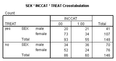
Page 449 Table 17.3
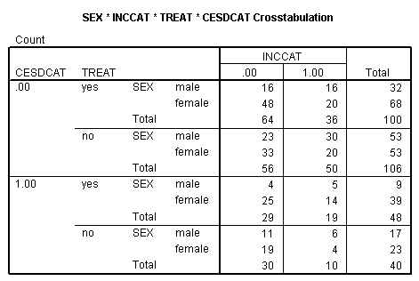
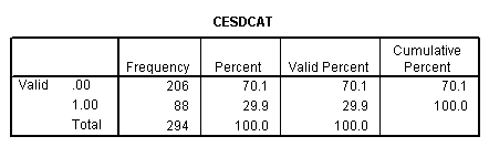
compute cesdcat = 0.
if cesd ge 11 cesdcat = 1.
crosstab sex by inccat by treat by cesdcat.
frequencies var = treat cesdcat sex inccat.
Page 451 middle of the page
crosstabs sex by inccat
 /cells = expected.
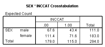
Page 454 top of the page
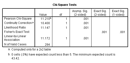
crosstabs sex by inccat
 /statistics = chisq.
<some output omitted>
Page 455 Table 17.7
if (sex=1) sex1=-1.
if (sex=2) sex1 =1.
if (inccat=0) inccat1=-1.
if (inccat=1) inccat1 =1.
compute sexinc = sex1*inccat1.
execute.

genlog  sex inccat with sex1 inccat1 sexinc
 /model = poisson
 /print = estim
 /plot = none
 /design inccat1 sex1 sexinc.
- - - - - - - - - - - - - - - - - - - - - - - - - - - - - - - - - - - - - - - -
GENERAL LOGLINEAR ANALYSIS
- - - - - - - - - - - - - - - - - - - - - - - - - - - - - - - - - - - - - - - -
Data Information
294 cases are accepted.
0 cases are rejected because of missing data.
294 weighted cases will be used in the analysis.
4 cells are defined.
0 structural zeros are imposed by design.
0 sampling zeros are encountered.
- - - - - - - - - - - - - - - - - - - - - - - - - - - - - - - - - - - - - - - -
Variable Information
Factor Levels Value
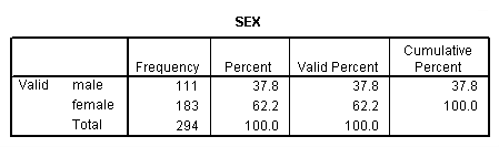
SEX 2
1.00 male
2.00 female
INCCAT 2
.00
1.00
- - - - - - - - - - - - - - - - - - - - - - - - - - - - - - - - - - - - - - - -
Covariates
SEX1
INCCAT1
SEXINC
- - - - - - - - - - - - - - - - - - - - - - - - - - - - - - - - - - - - - - - -
Model and Design Information
Model: Poisson
Design: Constant + INCCAT1 + SEX1 + SEXINC
- - - - - - - - - - - - - - - - - - - - - - - - - - - - - - - - - - - - - - - -
Correspondence Between Parameters and Terms of the Design
Parameter Aliased Term
1 Constant
2 INCCAT1
3 SEX1
4 SEXINC
- - - - - - - - - - - - - - - - - - - - - - - - - - - - - - - - - - - - - - - -
GENERAL LOGLINEAR ANALYSIS
- - - - - - - - - - - - - - - - - - - - - - - - - - - - - - - - - - - - - - - -
Convergence Information
Maximum number of iterations: 20
Relative difference tolerance: .001
Final relative difference: 9.12709E-14
Maximum likelihood estimation converged at iteration 1.
- - - - - - - - - - - - - - - - - - - - - - - - - - - - - - - - - - - - - - - -
Goodness-of-fit Statistics
Chi-Square DF Sig.
Likelihood Ratio .0000 0 .
Pearson .0000 0 .
- - - - - - - - - - - - - - - - - - - - - - - - - - - - - - - - - - - - - - - -
Parameter Estimates
Asymptotic 95% CI
Parameter Estimate SE Z-value Lower Upper
1 4.2378 .0616 68.75 4.12 4.36
2 -.1774 .0616 -2.88 -.30 -.06
3 .2128 .0616 3.45 .09 .33
4 -.2042 .0616 -3.31 -.33 -.08
Page 461
Row 3 comparing all two-factor association and first order terms with saturated model
genlog sex treat inccat
 /model = poisson
 /print=none
 /plot=none
 /design inccat*sex inccat*treat sex*treat.
- - - - - - - - - - - - - - - - - - - - - - - - - - - - - - - - - - - - - - - -
GENERAL LOGLINEAR ANALYSIS
- - - - - - - - - - - - - - - - - - - - - - - - - - - - - - - - - - - - - - - -
Data Information
294 cases are accepted.
0 cases are rejected because of missing data.
294 weighted cases will be used in the analysis.
8 cells are defined.
0 structural zeros are imposed by design.
0 sampling zeros are encountered.
- - - - - - - - - - - - - - - - - - - - - - - - - - - - - - - - - - - - - - - -
Variable Information
Factor Levels Value
SEX 2
1.00 male
2.00 female
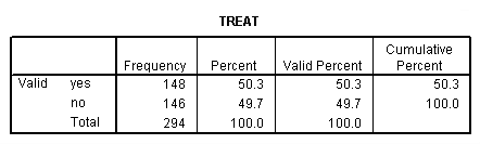
TREAT 2 Has a doctor prescribed or recommended that you take
1.00 yes
2.00 no
INCCAT 2
.00
1.00
- - - - - - - - - - - - - - - - - - - - - - - - - - - - - - - - - - - - - - - -
Model and Design Information
Model: Poisson
Design: Constant + SEX*INCCAT + TREAT*INCCAT + SEX*TREAT
- - - - - - - - - - - - - - - - - - - - - - - - - - - - - - - - - - - - - - - -
Correspondence Between Parameters and Terms of the Design
Parameter Aliased Term
1 Constant
2 [SEX = 1.00]*[INCCAT = .00]
3 [SEX = 1.00]*[INCCAT = 1.00]
4 [SEX = 2.00]*[INCCAT = .00]
5 x [SEX = 2.00]*[INCCAT = 1.00]
6 [TREAT = 1.00]*[INCCAT = .00]
7 [TREAT = 1.00]*[INCCAT = 1.00]
8 x [TREAT = 2.00]*[INCCAT = .00]
9 x [TREAT = 2.00]*[INCCAT = 1.00]
10 [SEX = 1.00]*[TREAT = 1.00]
11 x [SEX = 1.00]*[TREAT = 2.00]
12 x [SEX = 2.00]*[TREAT = 1.00]
Parameter Aliased Term
13 x [SEX = 2.00]*[TREAT = 2.00]
Note: 'x' indicates an aliased (or a redundant) parameter.
These parameters are set to zero.
- - - - - - - - - - - - - - - - - - - - - - - - - - - - - - - - - - - - - - - -
Convergence Information
Maximum number of iterations: 20
Relative difference tolerance: .001
Final relative difference: .0003
Maximum likelihood estimation converged at iteration 2.
- - - - - - - - - - - - - - - - - - - - - - - - - - - - - - - - - - - - - - - -
Goodness-of-fit Statistics
Chi-Square DF Sig.
Likelihood Ratio .0012 1 .9726
Pearson .0012 1 .9726
Row 2 comparing all first order terms with saturated
genlog sex treat inccat
 /model=poisson
 /print=none
 /plot=none
 /design inccat sex treat.
<some output omitted>
- - - - - - - - - - - - - - - - - - - - - - - - - - - - - - - - - - - - - - - -

Model and Design Information

 Model: Poisson
Design: Constant + INCCAT + SEX + TREAT

- - - - - - - - - - - - - - - - - - - - - - - - - - - - - - - - - - - - - - - -

Correspondence Between Parameters and Terms of the Design

Parameter   Aliased  Term

        1            Constant
        2            [INCCAT = .00]
        3       x    [INCCAT = 1.00]
        4            [SEX = 1.00]
        5       x    [SEX = 2.00]
        6            [TREAT = 1.00]
        7       x    [TREAT = 2.00]

Note: 'x' indicates an aliased (or a redundant) parameter.
      These parameters are set to zero.

- - - - - - - - - - - - - - - - - - - - - - - - - - - - - - - - - - - - - - - -
                          GENERAL LOGLINEAR ANALYSIS
- - - - - - - - - - - - - - - - - - - - - - - - - - - - - - - - - - - - - - - -

Convergence Information

Maximum number of iterations:            20
Relative difference tolerance:         .001
Final relative difference:      2.60437E-06

Maximum likelihood estimation converged at iteration 4.

- - - - - - - - - - - - - - - - - - - - - - - - - - - - - - - - - - - - - - - -

Goodness-of-fit Statistics

                    Chi-Square       DF       Sig.

Likelihood Ratio       24.0763        4     8.E-05
         Pearson       24.6519        4     6.E-05
Row 1 comparing the empty model with the model of all two-factor models
To obtain the comparison with row 2 of the table, subtract the value of row 2 from the model below. Note also that the degrees of freedom listed in the output is incorrect, showing one more than it should. This is because we had to add the extra constant term to the model to get it to run. (We were unable to figure out how to get SPSS genlog to run a constant only model, so we created a constant and used that in addition to the one SPSS used.)
compute cons = 0.
exe.
genlog sex treat inccat  with cons
  /model = poisson
  /print = none
  /plot = none
  /design cons.
- - - - - - - - - - - - - - - - - - - - - - - - - - - - - - - - - - - - - - - -

Model and Design Information

 Model: Poisson
Design: Constant + CONS

- - - - - - - - - - - - - - - - - - - - - - - - - - - - - - - - - - - - - - - -

Correspondence Between Parameters and Terms of the Design

Parameter   Aliased  Term

        1            Constant
        2       x    CONS

Note: 'x' indicates an aliased (or a redundant) parameter.
      These parameters are set to zero.

- - - - - - - - - - - - - - - - - - - - - - - - - - - - - - - - - - - - - - - -
                          GENERAL LOGLINEAR ANALYSIS
- - - - - - - - - - - - - - - - - - - - - - - - - - - - - - - - - - - - - - - -

Convergence Information

Maximum number of iterations:            20
Relative difference tolerance:         .001
Final relative difference:      8.68524E-06

Maximum likelihood estimation converged at iteration 4.

- - - - - - - - - - - - - - - - - - - - - - - - - - - - - - - - - - - - - - - -

Goodness-of-fit Statistics

                    Chi-Square       DF       Sig.

Likelihood Ratio       55.9474        7     1.E-09
         Pearson       61.3197        7     8.E-11
Page 462
hiloglinear sex(1 2) treat(1 2) inccat(0 1)
  /method=backward
  /print=none
  /design inccat*sex inccat*treat sex*treat.
* * * * * * * *  H I E R A R C H I C A L   L O G   L I N E A R  * * * * * * * *

DATA   Information

        294 unweighted cases accepted.
          0 cases rejected because of out-of-range factor values.
          0 cases rejected because of missing data.
        294 weighted cases will be used in the analysis.


FACTOR Information

   Factor  Level  Label
   SEX         2
   TREAT       2  Has a doctor prescribed or recom
   INCCAT      2

- - - - - - - - - - - - - - - - - - - - - - - - - - - - - - - - - - - - - - - -

* * * * * * * *  H I E R A R C H I C A L   L O G   L I N E A R  * * * * * * * *

Backward Elimination (p = .050) for DESIGN 1 with generating class

  INCCAT*SEX
  INCCAT*TREAT
  SEX*TREAT

 Likelihood ratio chi square =      .00118    DF = 1  P =  .973

- - - - - - - - - - - - - - - - - - - - - - - - - - - - - - - - - - - - - - - -

If Deleted Simple Effect is                 DF   L.R. Chisq Change    Prob  Iter

 INCCAT*SEX                                  1              10.669   .0011     2
 INCCAT*TREAT                                1                .000   .9934     2
 SEX*TREAT                                   1              12.451   .0004     2

Step 1

  The best model has generating class

      INCCAT*SEX
      SEX*TREAT

  Likelihood ratio chi square =      .00125    DF = 2  P =  .999

- - - - - - - - - - - - - - - - - - - - - - - - - - - - - - - - - - - - - - - -

If Deleted Simple Effect is                 DF   L.R. Chisq Change    Prob  Iter

 INCCAT*SEX                                  1              11.147   .0008     2
 SEX*TREAT                                   1              12.928   .0003     2

Step 2

  The best model has generating class

      INCCAT*SEX
      SEX*TREAT

  Likelihood ratio chi square =      .00125    DF = 2  P =  .999

- - - - - - - - - - - - - - - - - - - - - - - - - - - - - - - - - - - - - - - -

* * * * * * * *  H I E R A R C H I C A L   L O G   L I N E A R  * * * * * * * *

The final model has generating class

    INCCAT*SEX
    SEX*TREAT

The Iterative Proportional Fit algorithm converged at iteration 0.
The maximum difference between observed and fitted marginal totals is     .000
and the convergence criterion is     .250

- - - - - - - - - - - - - - - - - - - - - - - - - - - - - - - - - - - - - - - -


 Goodness-of-fit test statistics

    Likelihood ratio chi square =      .00125    DF = 2  P =  .999
             Pearson chi square =      .00125    DF = 2  P =  .999

- - - - - - - - - - - - - - - - - - - - - - - - - - - - - - - - - - - - - - - -
Page 463 The description of the stepwise analysis in the second half of the page.
hiloglinear inccat (0 1) sex1 (0 1) treat1 (0 1) cesdcat (0 1)
 /method = backward
 /maxorder=3
 /design = inccat*sex1*treat1*cesdcat.
* * * * * * * *  H I E R A R C H I C A L   L O G   L I N E A R  * * * * * * * *

DATA   Information

        294 unweighted cases accepted.
          0 cases rejected because of out-of-range factor values.
          0 cases rejected because of missing data.
        294 weighted cases will be used in the analysis.

FACTOR Information

   Factor  Level  Label
   INCCAT      2
   SEX1        2
   TREAT1      2
   CESDCAT     2

- - - - - - - - - - - - - - - - - - - - - - - - - - - - - - - - - - - - - - - -
* * * * * * * *  H I E R A R C H I C A L   L O G   L I N E A R  * * * * * * * *

Backward Elimination (p = .050) for DESIGN 1 with generating class

  INCCAT*SEX1*TREAT1
  INCCAT*SEX1*CESDCAT
  INCCAT*TREAT1*CESDCAT
  SEX1*TREAT1*CESDCAT

 Likelihood ratio chi square =      .04568    DF = 1  P =  .831
- - - - - - - - - - - - - - - - - - - - - - - - - - - - - - - - - - - - - - - -
If Deleted Simple Effect is                 DF   L.R. Chisq Change    Prob  Iter

 INCCAT*SEX1*TREAT1                          1                .008   .9294     4
 INCCAT*SEX1*CESDCAT                         1                .009   .9225     3
 INCCAT*TREAT1*CESDCAT                       1               4.742   .0294     2
 SEX1*TREAT1*CESDCAT                         1               1.227   .2681     3

Step 1
  The best model has generating class

      INCCAT*SEX1*CESDCAT
      INCCAT*TREAT1*CESDCAT
      SEX1*TREAT1*CESDCAT

  Likelihood ratio chi square =      .05353    DF = 2  P =  .974
- - - - - - - - - - - - - - - - - - - - - - - - - - - - - - - - - - - - - - - -
If Deleted Simple Effect is                 DF   L.R. Chisq Change    Prob  Iter

 INCCAT*SEX1*CESDCAT                         1                .011   .9173     3
 INCCAT*TREAT1*CESDCAT                       1               4.740   .0295     2
 SEX1*TREAT1*CESDCAT                         1               1.241   .2653     4

Step 2
  The best model has generating class

      INCCAT*TREAT1*CESDCAT
      SEX1*TREAT1*CESDCAT
      INCCAT*SEX1

  Likelihood ratio chi square =      .06431    DF = 3  P =  .996
- - - - - - - - - - - - - - - - - - - - - - - - - - - - - - - - - - - - - - - -
* * * * * * * *  H I E R A R C H I C A L   L O G   L I N E A R  * * * * * * * *

If Deleted Simple Effect is                 DF   L.R. Chisq Change    Prob  Iter

 INCCAT*TREAT1*CESDCAT                       1               4.986   .0256     3
 SEX1*TREAT1*CESDCAT                         1               1.239   .2656     3
 INCCAT*SEX1                                 1              10.495   .0012     2

Step 3
  The best model has generating class

      INCCAT*TREAT1*CESDCAT
      INCCAT*SEX1
      SEX1*TREAT1
      SEX1*CESDCAT

  Likelihood ratio chi square =     1.30361    DF = 4  P =  .861
- - - - - - - - - - - - - - - - - - - - - - - - - - - - - - - - - - - - - - - -
If Deleted Simple Effect is                 DF   L.R. Chisq Change    Prob  Iter

 INCCAT*TREAT1*CESDCAT                       1               4.273   .0387     3
 INCCAT*SEX1                                 1               9.783   .0018     3
 SEX1*TREAT1                                 1              11.853   .0006     3
 SEX1*CESDCAT                                1               2.218   .1364     3

Step 4
  The best model has generating class

      INCCAT*TREAT1*CESDCAT
      INCCAT*SEX1
      SEX1*TREAT1

  Likelihood ratio chi square =     3.52193    DF = 5  P =  .620
- - - - - - - - - - - - - - - - - - - - - - - - - - - - - - - - - - - - - - - -
If Deleted Simple Effect is                 DF   L.R. Chisq Change    Prob  Iter

 INCCAT*TREAT1*CESDCAT                       1               4.397   .0360     3
 INCCAT*SEX1                                 1              10.669   .0011     2
 SEX1*TREAT1                                 1              12.451   .0004     2
* * * * * * * *  H I E R A R C H I C A L   L O G   L I N E A R  * * * * * * * *
Step 5
  The best model has generating class

      INCCAT*TREAT1*CESDCAT
      INCCAT*SEX1
      SEX1*TREAT1

  Likelihood ratio chi square =     3.52193    DF = 5  P =  .620
- - - - - - - - - - - - - - - - - - - - - - - - - - - - - - - - - - - - - - - -
* * * * * * * *  H I E R A R C H I C A L   L O G   L I N E A R  * * * * * * * *

The final model has generating class

    INCCAT*TREAT1*CESDCAT
    INCCAT*SEX1
    SEX1*TREAT1

The Iterative Proportional Fit algorithm converged at iteration 0.
The maximum difference between observed and fitted marginal totals is     .083
and the convergence criterion is     .250
- - - - - - - - - - - - - - - - - - - - - - - - - - - - - - - - - - - - - - - -
 Observed, Expected Frequencies and Residuals.

       Factor          Code            OBS count  EXP count  Residual  Std Resid

  INCCAT                 0
   SEX1                   0
    TREAT1                 0
     CESDCAT                0               16.0       13.7      2.28        .62
     CESDCAT                1                4.0        6.2     -2.22       -.89
    TREAT1                 1
     CESDCAT                0               23.0       22.2       .82        .17
     CESDCAT                1               11.0       11.9      -.88       -.26
   SEX1                   1
    TREAT1                 0
     CESDCAT                0               48.0       50.3     -2.29       -.32
     CESDCAT                1               25.0       22.8      2.21        .46
    TREAT1                 1
     CESDCAT                0               33.0       33.8      -.81       -.14
     CESDCAT                1               19.0       18.1       .89        .21

  INCCAT                 1
   SEX1                   0
    TREAT1                 0
     CESDCAT                0               16.0       13.8      2.21        .60
     CESDCAT                1                5.0        7.3     -2.28       -.84
    TREAT1                 1
     CESDCAT                0               30.0       29.9       .05        .01
     CESDCAT                1                6.0        6.0       .01        .00
   SEX1                   1
    TREAT1                 0
     CESDCAT                0               20.0       22.2     -2.21       -.47

* * * * * * * *  H I E R A R C H I C A L   L O G   L I N E A R  * * * * * * * *

 Observed, Expected Frequencies and Residuals. (Cont.)

       Factor          Code            OBS count  EXP count  Residual  Std Resid

     CESDCAT                1               14.0       11.7      2.28        .67
    TREAT1                 1
     CESDCAT                0               20.0       20.1      -.06       -.01
     CESDCAT                1                4.0        4.0      -.01       -.01

- - - - - - - - - - - - - - - - - - - - - - - - - - - - - - - - - - - - - - - -
 Goodness-of-fit test statistics

    Likelihood ratio chi square =     3.52193    DF = 5  P =  .620
             Pearson chi square =     3.37768    DF = 5  P =  .642
- - - - - - - - - - - - - - - - - - - - - - - - - - - - - - - - - - - - - - - -
Page 464
NOTE: Because a /design subcommand was omitted, SPSS assumes a saturated model.
hiloglinear inccat (0 1) sex1 (0 1) treat1 (0 1) cesdcat (0 1)
  /print=all.
<some output omitted>
* * * * * * * *  H I E R A R C H I C A L   L O G   L I N E A R  * * * * * * * *

 Tests of PARTIAL associations.

  Effect Name                                    DF  Partial Chisq    Prob  Iter


  INCCAT*SEX1*TREAT1                              1           .008   .9294     4
  INCCAT*SEX1*CESDCAT                             1           .009   .9225     3
  INCCAT*TREAT1*CESDCAT                           1          4.742   .0294     2
  SEX1*TREAT1*CESDCAT                             1          1.227   .2681     3
  INCCAT*SEX1                                     1          9.906   .0016     3
  INCCAT*TREAT1                                   1           .002   .9653     3
  SEX1*TREAT1                                     1         11.976   .0005     3
  INCCAT*CESDCAT                                  1          1.168   .2799     4
  SEX1*CESDCAT                                    1          2.342   .1259     4
  TREAT1*CESDCAT                                  1           .317   .5733     4
  INCCAT                                          1         14.044   .0002     2
  SEX1                                            1         17.813   .0000     2
  TREAT1                                          1           .014   .9071     2
  CESDCAT                                         1         48.722   .0000     2

- - - - - - - - - - - - - - - - - - - - - - - - - - - - - - - - - - - - - - - -
Page 468
if (sex = 1) sex1= 1.
if (sex = 2) sex1 = -1.
if (treat =1) treat1 = 1.
if (treat = 2) treat1 = -1.
if (inccat = 0) inccat1 = -1.
if (inccat = 1) inccat1 = 1.
compute sextreat = sex1*treat1.
compute sexinc = sex1*inccat1.
compute treatinc = treat1*inccat1.
execute.

genlog sex inccat treat with sex1 inccat1 treat1 sexinc sextreat treatinc
 /model = poisson
 /print = estim
 /plot = none
 /design inccat1 sex1 sexinc sextreat treat1 treatinc.
- - - - - - - - - - - - - - - - - - - - - - - - - - - - - - - - - - - - - - - -
                          GENERAL LOGLINEAR ANALYSIS
- - - - - - - - - - - - - - - - - - - - - - - - - - - - - - - - - - - - - - - -

Data Information

       294 cases are accepted.
         0 cases are rejected because of missing data.
       294 weighted cases will be used in the analysis.
         8 cells are defined.
         0 structural zeros are imposed by design.
         0 sampling zeros are encountered.

- - - - - - - - - - - - - - - - - - - - - - - - - - - - - - - - - - - - - - - -

Variable Information

Factor     Levels    Value

SEX            2
                      1.00 male
                      2.00 female

INCCAT         2
                       .00
                      1.00

TREAT          2           Has a doctor prescribed or recommended that you take
                      1.00 yes
                      2.00 no

- - - - - - - - - - - - - - - - - - - - - - - - - - - - - - - - - - - - - - - -

Covariates
SEX1
INCCAT1
TREAT1
SEXINC
SEXTREAT
TREATINC

- - - - - - - - - - - - - - - - - - - - - - - - - - - - - - - - - - - - - - - -

Model and Design Information

 Model: Poisson
Design: Constant + INCCAT1 + SEX1 + SEXINC + SEXTREAT + TREAT1 + TREATINC

- - - - - - - - - - - - - - - - - - - - - - - - - - - - - - - - - - - - - - - -
                          GENERAL LOGLINEAR ANALYSIS
- - - - - - - - - - - - - - - - - - - - - - - - - - - - - - - - - - - - - - - -

Correspondence Between Parameters and Terms of the Design

Parameter   Aliased  Term

        1            Constant
        2            INCCAT1
        3            SEX1
        4            SEXINC
        5            SEXTREAT
        6            TREAT1
        7            TREATINC

- - - - - - - - - - - - - - - - - - - - - - - - - - - - - - - - - - - - - - - -

Convergence Information

Maximum number of iterations:            20
Relative difference tolerance:         .001
Final relative difference:            .0003

Maximum likelihood estimation converged at iteration 2.

- - - - - - - - - - - - - - - - - - - - - - - - - - - - - - - - - - - - - - - -

Goodness-of-fit Statistics

                    Chi-Square       DF       Sig.

Likelihood Ratio         .0012        1      .9726
         Pearson         .0012        1      .9726

- - - - - - - - - - - - - - - - - - - - - - - - - - - - - - - - - - - - - - - -
                          GENERAL LOGLINEAR ANALYSIS
- - - - - - - - - - - - - - - - - - - - - - - - - - - - - - - - - - - - - - - -

Parameter Estimates

                                               Asymptotic 95% CI
Parameter   Estimate         SE    Z-value      Lower      Upper

        1     3.5121      .0636      55.25       3.39       3.64
        2     -.1784      .0620      -2.88       -.30       -.06
        3     -.2246      .0636      -3.53       -.35       -.10
        4      .2056      .0633       3.25        .08        .33
        5     -.2194      .0630      -3.48       -.34       -.10
        6     -.0481      .0627       -.77       -.17        .07
        7      .0005      .0623  8.324E-03       -.12        .12
Page 470 top of the page
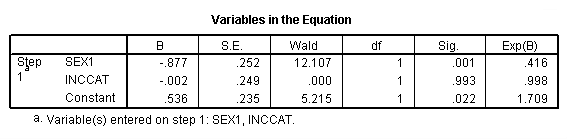
get file 'c:cama4depress.sav'.
compute sex1 = sex - 1.
compute treat1 = treat - 1.
logistic regression var = treat1 with sex1, inccat.