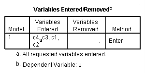
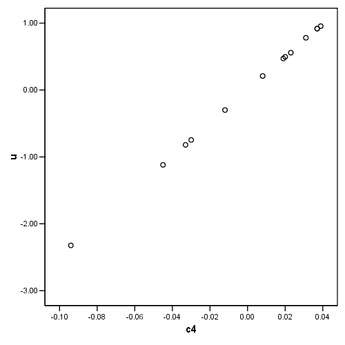
Table 10.1, Page 265. Regression results of fitting model (10.2) to the Import Data (1949-1959).
get file 'd:p233.sav'.
select if (year <= 59).
exe.
The analysis requires the dependent variable be converted into its standardized value. This is done using the descriptive command using the save option.
descriptives variable = import
 /save.
[output omitted]
regression
/dependent = zimport
/method enter = doprod stock consum.
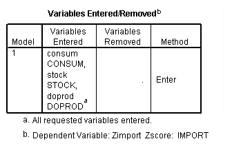
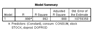


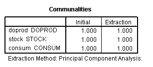
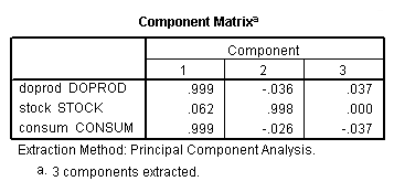
Table 10.2, page 265. Regression results of fitting model (10.5) to the
Import Data (1949-1959).
Analysis requires calculation of principal component scores. SPSS does not
calculate PC scores, rather it uses factor scores. There is a direct linear
relationship between the
two scores and the standardized regression coefficients are equivalent.
factor variables = doprod stock consum
 /criteria factors(3) iterate(25)
 /extraction pc
 /rotation norate
 /save reg( 3, fs).

regression
 /dependent = zimport
 /method enter = fs1 fs2 fs3.
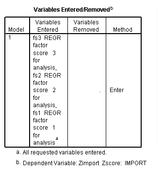
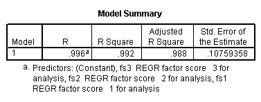
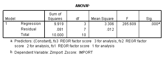
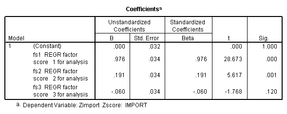
Table 10.4, page 270. A response variable U and a set of principal components of four predictor variables.
get file 'd:p270.sav'.
list.
        u        c1        c2        c3        c4

      .95      1.47      1.90      -.53       .04
     -.75      2.14       .24      -.29      -.03
    -2.32     -1.13       .18      -.01      -.09
     -.82       .66      1.58       .18      -.03
      .47      -.36       .48      -.74       .02
     -.30      -.97       .17       .09      -.01
      .21      -.93     -2.13      -.17       .01
      .56      2.23      -.69       .46       .02
    -1.12       .35     -1.43      -.03      -.05
      .50     -1.66      1.83       .85       .02
      .78      1.64     -1.29       .49       .03
      .92     -1.69      -.39      -.02       .04
      .92     -1.75      -.44      -.28       .04

Number of cases read:  13    Number of cases listed:  13
Table 10.5, page 270. Regression results using all four PCs of Hald’s data.
NOTE: The value for the regression coefficients and t-test for c4 are slightly off.
regression
 /dependent = u
 /method enter = c1 c2 c3 c4.


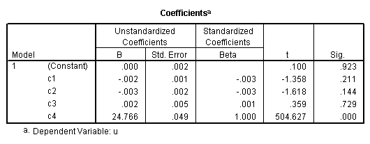
Table 10.6, page 270. Regression results using the first three PCs of Hald’s data.
regression
 /dependent = u
 /method enter = c1 c2 c3.
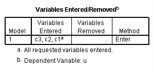


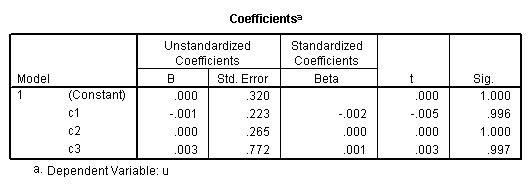
Figure 10.1, page 271. Scatter plots of U versus each of the PCs of the Hald’s data.
graph
 /scatterplot = c1 with u.
graph
 /scatterplot = c2 with u.
graph
 /scatterplot = c3 with u.
graph
 /scatterplot = c4 with u.

