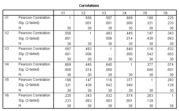
Table 11.1, page 295. Correlation Matrix for the Supervision Performance Data in Table 3.3.
get file 'd:p054.sav'.
correlation variables = x1 x2 x3 x4 x5 x6.
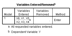
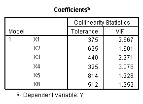
VIF, middle of page 295.
regression
 /statistics tol
 /dependent = y
 /method enter = x1 x2 x3 x4 x5 x6.
Eigenvalues, bottom of page 295.
factor variables = x1 x2 x3 x4 x5 x6
 /criteria factors (6)
 /rotation norotate
 /method = correlation.
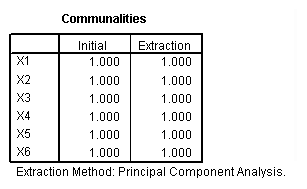
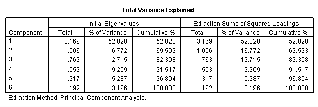
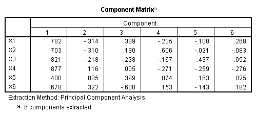
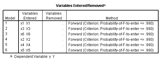
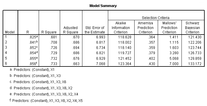
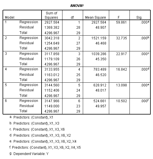
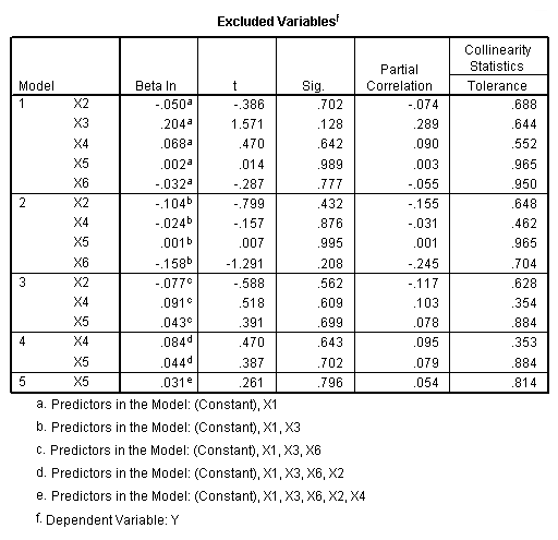
Table 11.2, page 296. Variables selected by the Forward Selection Method.
NOTE: The probability (p-value) for entering was set at .99 so that all the
variables will be entered into the model. The reason is that we are mainly
interested in the order in which they entered the model.
regression
 /statistics = selection coef outs r anova
 /criteria = pin(.99) pout(.1)
 /dependent = y
 /method = forward x1 x2 x3 x4 x5 x6.
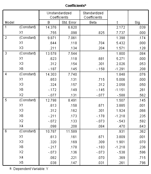
Regression Equation, page 296.
NOTE: The probability to remove, pout(.33) corresponds to a t-value of 1.0.
regression
 /statistics = coef
 /criteria = pin(.1) pout(.33)
 /dependent = y
 /method = backward x1 x2 x3 x4 x5 x6.
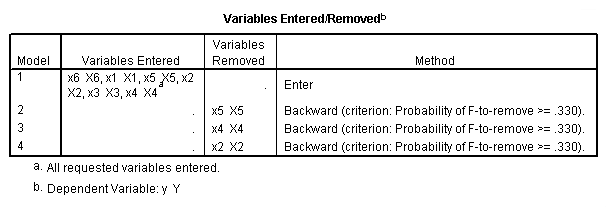
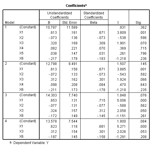
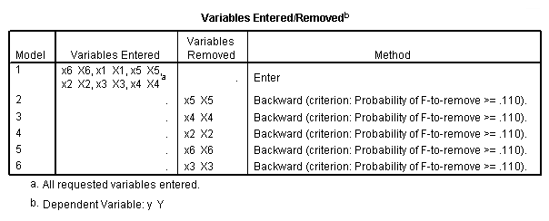
Table 11.3, page 297. Variables selected by the Backward Elimination Method.
NOTE: The probability (p-value) for removal was set at .01 so that all the
variables will be entered into the model.
regression
 /statistics = selection coef outs r anova
 /criteria = pin(.1) pout(.01)
 /dependent = y
 /method = backward x1 x2 x3 x4 x5 x6.
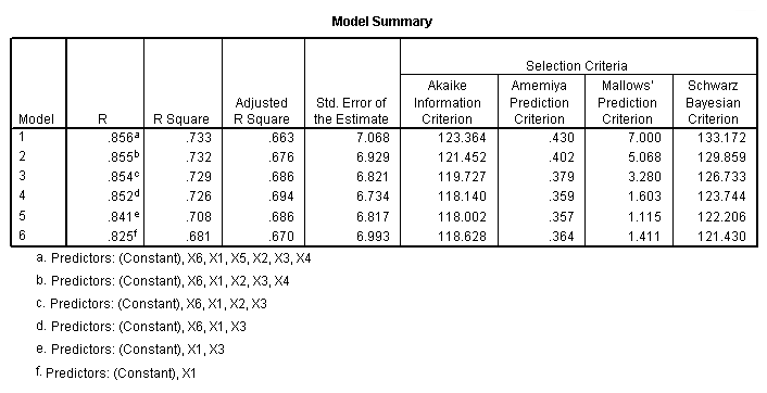
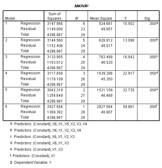
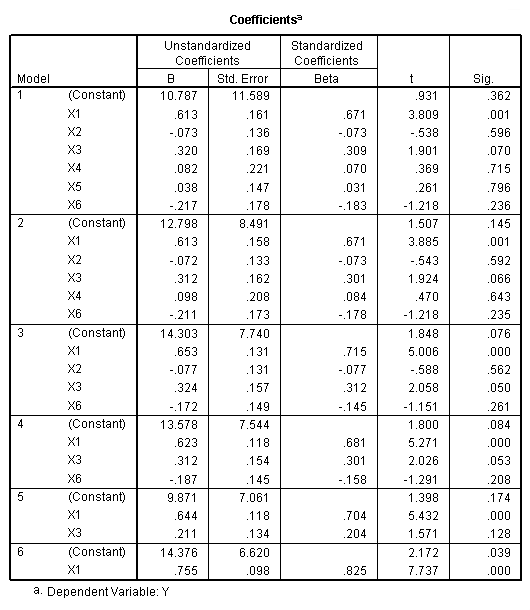
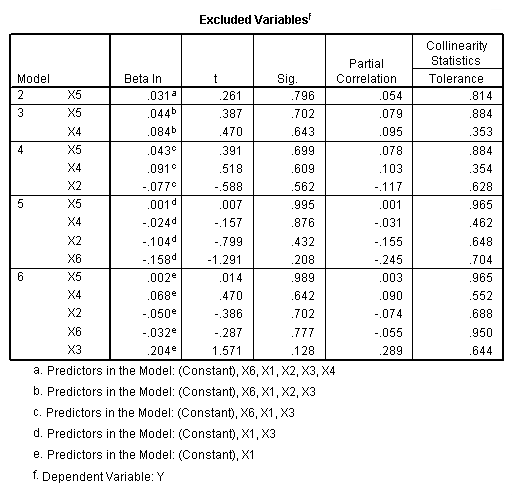
Table 11.4-11.5 page 297and Figure 11.1 page 298.
NOTE: SPSS does not have the best subset option.
Table 11.7, page 301. First Part of the Homicide Data.
get file 'd:p301.sav'.
list variables year to clear.
    year       ftp     unemp         m       lic        gr     clear

    1961    260.35     11.00    455.50    178.15    215.98     93.40
    1962    269.80      7.00    480.20    156.41    180.48     88.50
    1963    272.04      5.20    506.10    198.02    209.57     94.40
    1964    272.96      4.30    535.80    222.10    231.67     92.00
    1965    272.51      3.50    576.00    301.92    297.65     91.00
    1966    261.34      3.20    601.70    391.22    367.62     87.40
    1967    268.89      4.10    577.30    665.56    616.54     88.30
    1968    295.99      3.90    596.90   1131.21   1029.75     86.10
    1969    319.87      3.60    613.50    837.80    786.23     79.00
    1970    341.43      7.10    569.30    794.90    713.77     73.90
    1971    356.59      8.40    548.80    817.74    750.43     63.40
    1972    376.69      7.70    563.40    583.17   1027.38     62.50
    1973    390.19      6.30    609.30    709.59    666.50     58.90

Number of cases read:  13    Number of cases listed:  13
Table 11.8, page 301. Second Part of the Homicide Data.
list variables year w to h.
    year            w      nman         g        he        we         h

    1961       558724    538.10    133.90      2.98    117.18      8.60
    1962       538584    547.60    137.60      3.09    134.02      8.90
    1963       519171    562.80    143.60      3.23    141.68      8.52
    1964       500457    591.00    150.30      3.33    147.98      8.89
    1965       482418    626.10    164.30      3.46    159.85     13.07
    1966       465029    659.80    179.50      3.60    157.19     14.57
    1967       448267    686.20    187.50      3.73    155.29     21.36
    1968       432109    699.60    195.40      2.91    131.75     28.03
    1969       416533    729.90    210.30      4.25    178.74     31.49
    1970       401518    757.80    223.80      4.47    178.30     37.39
    1971       398046    755.30    227.70      5.04    209.54     46.26
    1972       373095    787.00    230.90      5.47    240.05     47.24
    1973       359647    819.80    230.20      5.76    258.05     52.33

Number of cases read:  13    Number of cases listed:  13
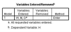
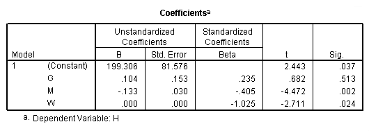
Table 11.9, page 301. The OLS Results From Fitting Model (11.8).
regression
 /statistics tol coef r
 /dependent = h
 /method enter = g m w.


Table 11.10, page 302.
Model A.
regression
 /statistics coef r
 /dependent = h
 /method enter = g.


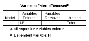
Model B.
regression
 /statistics coef r
 /dependent = h
 /method enter = m.


Model C.
regression
 /statistics coef r
 /dependent = h
 /method enter = w.


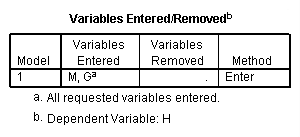
Model D.
regression
 /statistics coef r
 /dependent = h
 /method enter = g m.


Model E.
regression
 /statistics coef r
 /dependent = h
 /method enter = g w.


Model F.
regression
 /statistics coef r
 /dependent = h
 /method enter = g m w.


Model G.
regression
 /statistics coef r
 /dependent = h
 /method enter = m w.
