Table 2.3, page 25: A data set with a perfect nonlinear relationship between Y and X, yet Cor(X,Y) = 0
get file 'D:p025a.sav'.
list.
       y        x

       1       -7
      14       -6
      25       -5
      34       -4
      41       -3
      46       -2
      49       -1
      50        0
      49        1
      46        2
      41        3
      34        4
      25        5
      14        6
       1        7

Number of cases read:  15    Number of cases listed:  15
Figure 2.2, page 25: A scatter plot of Y versus X in Table 2.3
graph
/scatter = x with y.
Table 2.4, page 25 Anscombe’s Quartet: Four data sets having same values of summary statistics
get file 'D:p025b.sav'.
list.

       y1       x1        y2       x2        y3       x3        y4       x4

     8.04       10      9.14       10      7.46       10      6.58        8
     6.95        8      8.14        8      6.77        8      5.76        8
     7.58       13      8.74       13     12.74       13      7.71        8
     8.81        9      8.77        9      7.11        9      8.84        8
     8.33       11      9.26       11      7.81       11      8.47        8
     9.96       14      8.10       14      8.84       14      7.04        8
     7.24        6      6.13        6      6.08        6      5.25        8
     4.26        4      3.10        4      5.39        4     12.50       19
    10.84       12      9.13       12      8.15       12      5.56        8
     4.82        7      7.26        7      6.42        7      7.91        8
     5.68        5      4.74        5      5.73        5      6.89        8

Number of cases read:  11    Number of cases listed:  11
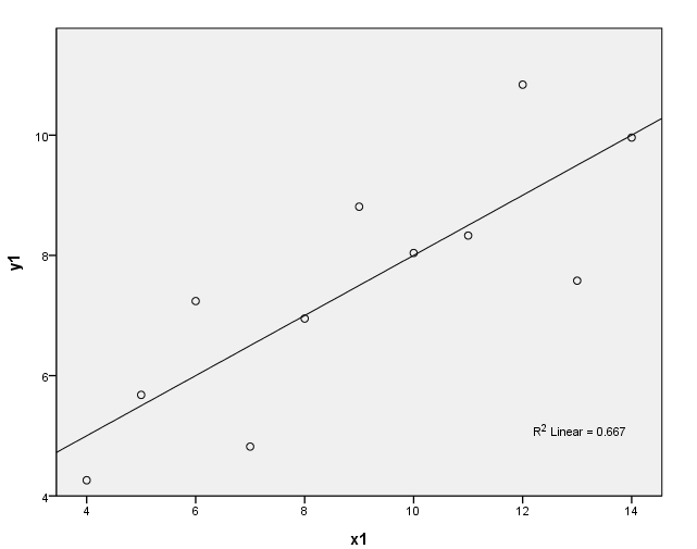
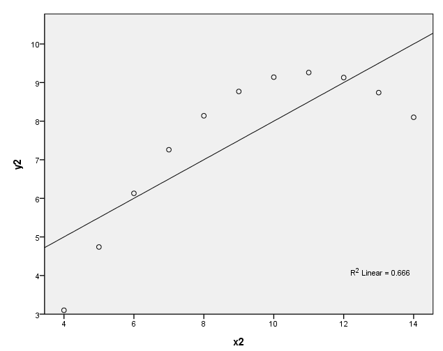
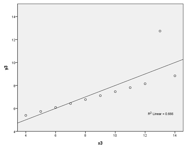
Figure 2.3, page 26: Scatter plots of the data in Table 2.4 with the fitted lines
graph (a)
formats y1 x1 y2 x2 y3 x3 y4 x4 (f2.0).
GGRAPH
  /GRAPHDATASET NAME="GraphDataset" VARIABLES= y1 x1
  /GRAPHSPEC SOURCE=INLINE
      INLINETEMPLATE=["<addFitLine  type='linear' target='pair'/> " ].
BEGIN GPL
SOURCE: s=userSource( id( "GraphDataset" ) )
DATA: y1=col( source(s), name( "y1" ) )
DATA: x1=col( source(s), name( "x1" ) )
GUIDE: axis( dim( 1 ), label( "x1" ) )
GUIDE: axis( dim( 2 ), label( "y1" ) )
ELEMENT: point( position( ( X1_Var * Y_Var ) ) )
END GPL.
graph (b)
GGRAPH
  /GRAPHDATASET NAME="GraphDataset" VARIABLES= y2 x2
  /GRAPHSPEC SOURCE=INLINE  INLINETEMPLATE=["<addFitLine  type='linear' target='pair'/> "].
BEGIN GPL
SOURCE: s=userSource( id( "GraphDataset" ) )
DATA: y2=col( source(s), name( "y2" ) )
DATA: x2=col( source(s), name( "x2" ) )
GUIDE: axis( dim( 1 ), label( "x2" ) )
GUIDE: axis( dim( 2 ), label( "y2" ) )
ELEMENT: point( position( (x2 * y2 ) ) )
END GPL.
graph (c)
GGRAPH
  /GRAPHDATASET NAME="GraphDataset" VARIABLES= y3 x3
  /GRAPHSPEC SOURCE=INLINE INLINETEMPLATE=["<addFitLine  type='linear' target='pair'/> " ].
BEGIN GPL
SOURCE: s=userSource( id( "GraphDataset" ) )
DATA: y3=col( source(s), name( "y3" ) )
DATA: x3=col( source(s), name( "x3" ) )
GUIDE: axis( dim( 1 ), label( "x3" ) )
GUIDE: axis( dim( 2 ), label( "y3" ) )
ELEMENT: point( position( ( x3 * y3 ) ) )
END GPL.
graph (d)
GGRAPH
  /GRAPHDATASET NAME="GraphDataset" VARIABLES= y4 x4
  /GRAPHSPEC SOURCE=INLINE INLINETEMPLATE=["<addFitLine  type='linear' target='pair'/> "].
BEGIN GPL
SOURCE: s=userSource( id( "GraphDataset" ) )
DATA: y4=col( source(s), name( "y4" ) )
DATA: x4=col( source(s), name("x4") )
GUIDE: axis( dim( 1 ), label( "x4" ) )
GUIDE: axis( dim( 2 ), label( "y4" ) )
ELEMENT: point( position( ( x4 * y4 ) ) )
END GPL.
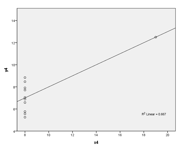
Table 2.5, page 27 length of service calls (in minutes) and number of units repaired
get file 'D:p027.sav'.
list.
 minutes    units

      23        1
      29        2
      49        3
      64        4
      74        4
      87        5
      96        6
      97        6
     109        7
     119        8
     149        9
     145        9
     154       10
     166       10

Number of cases read:  14    Number of cases listed:  14
Table 2.6, Page 28: Quantities needed for the computation of the correlation
coefficient between the
length of service calls, Y and the number of units repaired, X
compute const = 1.
exe.
aggregate outfile "d:p027ag.sav"
 /break =const
 /ymean = mean(minutes)
 /xmean = mean(units).
match files file =  *
 /table = "d:p027ag.sav"
 /by const.
exe.
compute yd = minutes - ymean.
compute xd = units - xmean.
compute yd2 = yd**2.
compute xd2 = xd**2.
compute xyd = xd*yd.
exe.
list minutes units yd to xyd.

 minutes    units       yd       xd      yd2      xd2      xyd

      23        1   -74.21    -5.00  5507.76    25.00   371.07
      29        2   -68.21    -4.00  4653.19    16.00   272.86
      49        3   -48.21    -3.00  2324.62     9.00   144.64
      64        4   -33.21    -2.00  1103.19     4.00    66.43
      74        4   -23.21    -2.00   538.90     4.00    46.43
      87        5   -10.21    -1.00   104.33     1.00    10.21
      96        6    -1.21      .00     1.47      .00      .00
      97        6     -.21      .00      .05      .00      .00
     109        7    11.79     1.00   138.90     1.00    11.79
     119        8    21.79     2.00   474.62     4.00    43.57
     149        9    51.79     3.00  2681.76     9.00   155.36
     145        9    47.79     3.00  2283.47     9.00   143.36
     154       10    56.79     4.00  3224.62    16.00   227.14
     166       10    68.79     4.00  4731.47    16.00   275.14

Number of cases read:  14    Number of cases listed:  14

descriptive variables = minutes to xyd
 /statistics = sum.
Figure 2.4, page 26 computer repair data: scatter plot of minutes versus units
graph
 /scatter units with minutes.
Table 2.7, page 32 the fitted values of, yhat, and the ordinary least squares residuals, e, for the repair data
regression
 /dependent = minutes
 /method = enter units
 /save resid (e) pred (yhat) sepred (semu).
list units yhat e.
   units        yhat           e

       1    19.67043     3.32957
       2    35.17920    -6.17920
       3    50.68797    -1.68797
       4    66.19674    -2.19674
       4    66.19674     7.80326
       5    81.70551     5.29449
       6    97.21429    -1.21429
       6    97.21429     -.21429
       7   112.72306    -3.72306
       8   128.23183    -9.23183
       9   143.74060     5.25940
       9   143.74060     1.25940
      10   159.24937    -5.24937
      10   159.24937     6.75063

Number of cases read:  14    Number of cases listed:  14
Figure 2.5, page 32 plot of minutes versus units with the fitted least squares regression line
GGRAPH
  /GRAPHDATASET NAME="GraphDataset" VARIABLES= minutes units
  /GRAPHSPEC SOURCE=INLINE
      INLINETEMPLATE=["<addFitLine  type='linear' target='pair'/> "].
BEGIN GPL
SOURCE: s=userSource( id( "GraphDataset" ) )
DATA: minutes=col( source(s), name( "minutes" ) )
DATA: units=col( source(s), name( "units" ) )
GUIDE: axis( dim( 1 ), label( "units" ) )
GUIDE: axis( dim( 2 ), label( "minutes" ) )
ELEMENT: point( position( ( units * minutes ) ) )
END GPL.
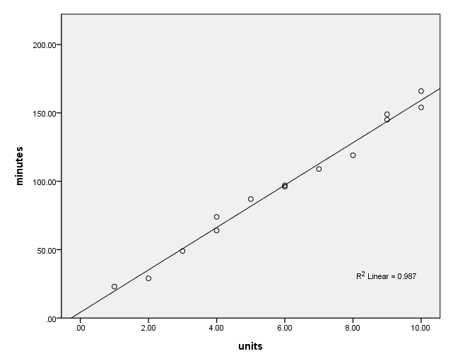
Table 2.8, page 36 regression output for the computer repair data
regression
 /statistics coef
 /dependent = minutes
 /method = enter units.
Standard error for mean prediction, page 39
list units minutes semu.
   units  minutes        semu

       1       23     2.90717
       2       29     2.48124
       3       49     2.09082
       4       64     1.75969
       4       74     1.75969
       5       87     1.52692
       6       96     1.44100
       6       97     1.44100
       7      109     1.52692
       8      119     1.75969
       9      149     2.09082
       9      145     2.09082
      10      154     2.48124
      10      166     2.48124

Number of cases read:  14    Number of cases listed:  14
Correlations, page 43
correlations variables = minutes units yhat.
NOTE: (.994)^2 = .987 = R^2