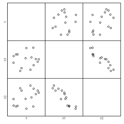
Figure 4.1, page 95 .
Duplicating Figure 2.3 from Chapter 2
get file 'D:p095.sav'.
graph
 /scatterplot(matrix) = y x1 x2.
correlations variables = y x1 x2.
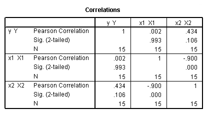
Table 4.2, page 95: Hamilton’s (1987) data
list.
y x1 x2

12.37 2.23 9.66
12.66 2.57 8.94
12.00 3.87 4.40
11.93 3.10 6.64
11.06 3.39 4.91
13.03 2.83 8.52
13.13 3.02 8.04
11.44 2.14 9.05
12.86 3.04 7.71
10.84 3.26 5.11
11.20 3.39 5.05
11.56 2.35 8.51
10.83 2.76 6.59
12.63 3.90 4.90
12.46 3.16 6.96

Number of cases read: 15 Number of cases listed: 15
Regression coefficients for page 95.
regression
 /dependent = y
 /method enter = x1.


regression
 /dependent = y
 /method enter = x2.
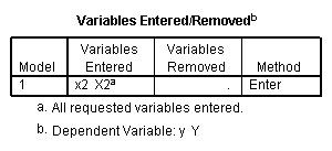


regression
 /dependent = y
 /method enter = x1 x2.
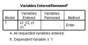


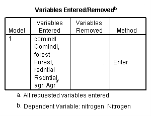
Table 4.2, page 99: New York Rivers Data: The t-test for the individual coefficients. None of the observations deleted.
get file 'D:p010.sav'.
regression
 /dependent = nitrogen
 /method enter = agr forest rsdntial comindl.
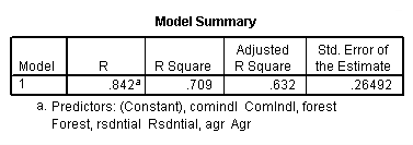


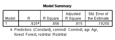
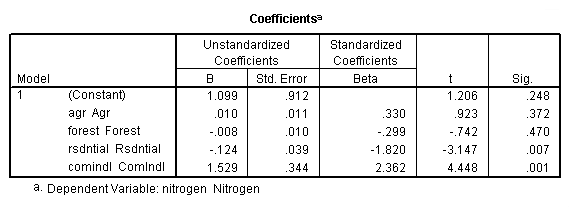
Neversink deleted.
temporary.
select if (river ~= "Neversink").
regression
 /dependent = nitrogen
 /method enter = agr forest rsdntial comindl.
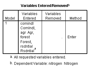

Hackensack deleted
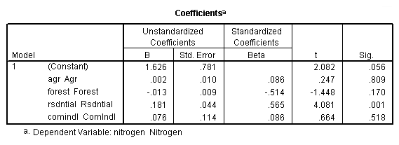
temporary.
select if (river ~= "Hackensack").
regression
 /dependent = nitrogen
 /method enter = agr forest rsdntial comindl.


Equation (4.18), page 102: also generate the residual and leverage for Table 4.3 and Figure 4.6
regression
 /dependent = nitrogen
 /method enter = comindl
 /save sresid(ri) lever(pi).
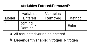
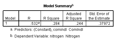


Figure 4.5, page 102: New York Rivers Data: Scatter plot of Y versus X4
compute i = $casenum.
exe.
formats i (f2.0).
GGRAPH
  /GRAPHDATASET NAME="GraphDataset" VARIABLES= nitrogen comindl i
  /GRAPHSPEC SOURCE=INLINE
      INLINETEMPLATE=["<addFitLine  type='linear' target='pair'/> " ].
BEGIN GPL
SOURCE: s=userSource( id( "GraphDataset" ) )
DATA: nitrogen=col( source(s), name( "nitrogen" ) )
DATA: comindl=col( source(s), name( "comindl" ) )
DATA: PointLabel = col( source(s), name( "i" ), unit.category() )
GUIDE: axis( dim( 1 ), label( "comindl" ) )
GUIDE: axis( dim( 2 ), label( "nitrogen" ) )
SCALE: linear( dim( 1 ), min(0.1), max(3.1) )
SCALE: linear( dim( 2 ), min(0.5), max(2.5) )
ELEMENT: point( position( comindl * nitrogen ), label( PointLabel ) )
END GPL.
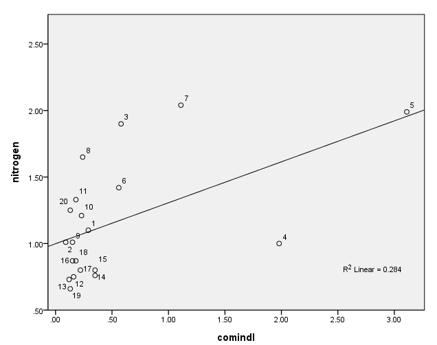
Table 4.3, page 103: New York Rivers Data: The standardized residuals, ri, and the leverage values, pii from fitting model 4.18.
NOTE: The leverage values do not match the book since they are calculated as the centered leverage values.
list i ri pi.
       i          ri          pi

    1.00      .03228      .00469
    2.00     -.04502      .01670
    3.00     1.95292      .00038
    4.00    -1.84723      .19787
    5.00      .15529      .62101
    6.00      .67231      .00018
    7.00     1.92326      .03261
    8.00     1.56562      .00700
    9.00     -.09515      .01232
   10.00      .38082      .00752
   11.00      .74924      .01038
   12.00     -.81033      .01166
   13.00     -.83246      .01443
   14.00     -.82939      .00253
   15.00     -.93761      .00253
   16.00     -.47590      .01232
   17.00     -.72323      .00806
   18.00     -.50049      .01038
   19.00    -1.03103      .01371
   20.00      .57473      .01371

Number of cases read:  20    Number of cases listed:  20
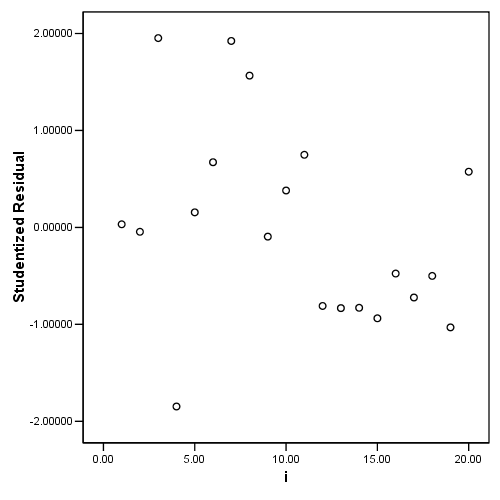
Figure 4.6, page 103: Index plots of (a) the standardized residuals, ri and (b) the leverage values pi.
(a)
graph
 /scatterplot= i with ri.
(b)
graph
 /scatterplot = i with pi.
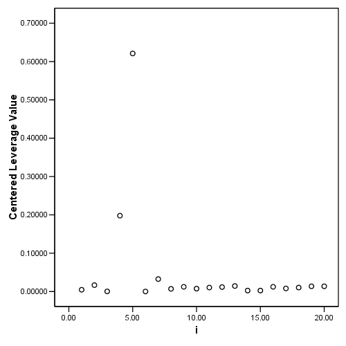
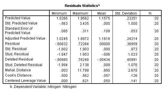
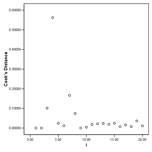
Table 4.4 and Figure 4.7 page 106
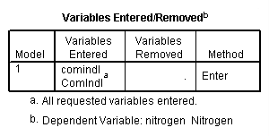
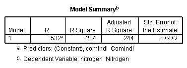
regression
 /dependent = nitrogen
 /method enter = comindl
 /save cook(c) dffit(dfits) resid(e).


Compute hadi. Since hadi is constructed using the leverage and not getting accurate leverage numbers, not calculating hadi.
compute d = e/1.6110.
compute hadi = (pi/(1-pi)) +((2)/(1-pi))*(d**2/(1-d**2)) .
exe.
list i c dfits hadi.
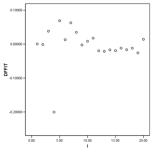
       i           c       dfits     hadi

    1.00      .00003      .00069      .00
    2.00      .00007     -.00118      .02
    3.00      .10118      .03834      .50
    4.00      .56225     -.20047      .66
    5.00      .02459      .06898     1.64
    6.00      .01194      .01315      .05
    7.00      .16653      .06299      .51
    8.00      .07408      .03490      .30
    9.00      .00030     -.00233      .01
   10.00      .00443      .00857      .02
   11.00      .01804      .01772      .07
   12.00      .02157     -.01959      .08
   13.00      .02386     -.02106      .09
   14.00      .01907     -.01699      .08
   15.00      .02437     -.01921      .10
   16.00      .00753     -.01163      .04
   17.00      .01612     -.01643      .06
   18.00      .00805     -.01184      .04
   19.00      .03617     -.02578      .13
   20.00      .01124      .01437      .05

Number of cases read:  20    Number of cases listed:  20
graph (a)
graph
 /scatterplot = i with c.
graph (b)
graph
 /scatterplot = i with dfits.
graph (c)
graph
 /scatterplot = i with hadi.
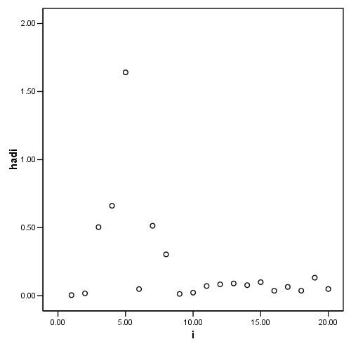
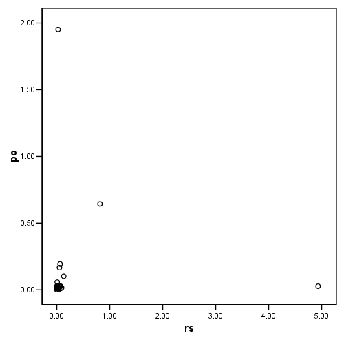
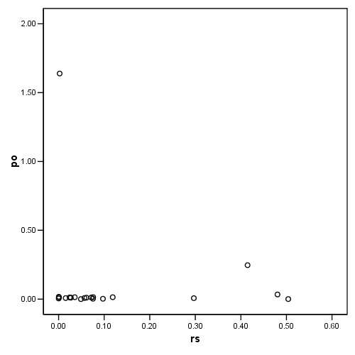
Figure 4.8, page 108: Potential-Residual Plot
compute po = (pi/(1-pi)).
compute rs =  ((2)/(1-pi))*(d**2/(1-d**2)).
exe.
graph
 /scatterplot = rs with po.
Equation (4.25), bottom of page 111
get file 'D:p112.sav'.
regression
 /dependent = time
 /method enter = distance climb.
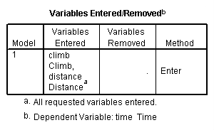


Table 4.5, page 112: Scottish Hills Race Data
list.

hillrace                      time  distance    climb

Greenmantle New Year Dash      965      2.50      650
Carnethy                      2901      6.00     2500
Craig Dunain                  2019      6.00      900
Ben Rha                       2736      7.50      800
Ben Lomond                    3736      8.00     3070
Goatfell                      4393      8.00     2866
Bens of Jura                 12277     16.00     7500
Cairnpapple                   2182      6.00      800
Scolty                        1785      5.00      800
Traprain Law                  2385      6.00      650
Lairig Ghru                  11560     28.00     2100
Dollar                        2583      5.00     2000
Lomonds of Fife               3900      9.50     2200
Cairn Table                   2648      6.00      500
Eildon Two                    1616      4.50     1500
Cairngorm                     4335     10.00     3000
Seven Hills of Edinburgh      5905     14.00     2200
Knock Hill                    4719      3.00      350
Black Hill                    1045      4.50     1000
Creag Beag                    1954      5.50      600
Kildoon                        957      3.00      300
Meall Ant-Suiche              1674      3.50     1500
Half Ben Nevis                2859      6.00     2200
Cow Hill                      1076      2.00      900
North Berwick Law             1121      3.00      600
Creag Dubh                    1573      4.00     2000
Burnswark                     2066      6.00      800
Largo                         1714      5.00      950
Criffel                       3030      6.50     1750
Achmony                       1257      5.00      500
Ben Nevis                     5135     10.00     4400
Knockfarrel                   1943      6.00      600
Two Breweries Fell           10215     18.00     5200
Cockleroi                     1686      4.50      850
Moffat Chase                  9590     20.00     5000

Number of cases read:  35    Number of cases listed:  35
Figure 4.10, page 113. Rotating plot for the Scottish Hills Race Data
compute id = $casenum.
exe.
formats id (f2.0).
GGRAPH
  /GRAPHDATASET NAME="GraphDataset" VARIABLES= time distance climb id
  /GRAPHSPEC SOURCE=INLINE
      INLINETEMPLATE=["<addDataLabels><labeling variable='percent'><format suffix='%'/></labeling></addDataLabels>"].
BEGIN GPL
SOURCE: s=userSource( id( "GraphDataset" ) )
DATA: time=col( source(s), name( "time" ) )
DATA: distance=col( source(s), name( "distance" ) )
DATA: climb=col( source(s), name( "climb" ) )
DATA: id = col( source(s), name( "id" ), unit.category() )
COORD: rect( dim( 1,2,3 ) )
GUIDE: axis( dim( 1 ), label( "climb" ), start(0.0), delta(8000))
GUIDE: axis( dim( 2 ), label( "distance" ), start(0.0), delta(30) )
GUIDE: axis( dim( 3 ), label( "time" ), start(0.0), delta(12000) )
SCALE: linear( dim( 1 ),  min(0), max(8000)  )
SCALE: linear( dim( 2 ), min(0), max(30) )
SCALE: linear( dim( 3 ), min(0), max(12000) )
ELEMENT: point( position( ( climb * distance * time ) ), label( id ) )
END GPL.
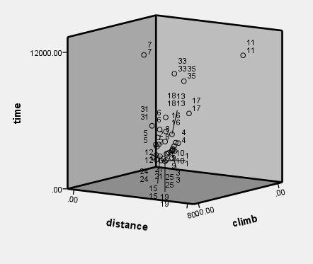
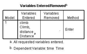
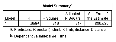
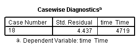
Figure 4.11, page 114. Added-variable plots for (a) distance and (b) climb
regression
 /dependent = time
 /method enter = distance climb
 /partialplot all
 /save resid(e) lever(pi).


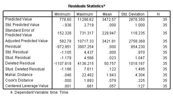
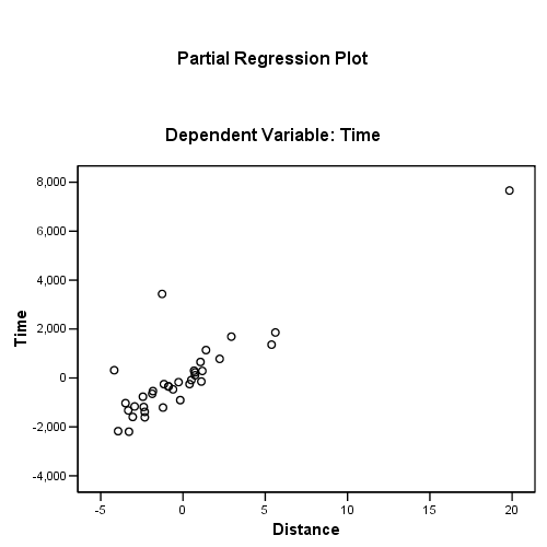
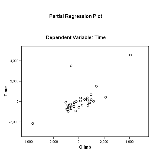
using the regression coefficients for calculating the residual plus component plot
compute rpc_dist = e + 373.073*distance.
compute rpc_climb = e + .663*climb.
exe.
Figure 4.12(a), page 114
Note: The graph in the book is incorrect; please see errata.
graph
 /scatterplot = distance with rpc_dist.
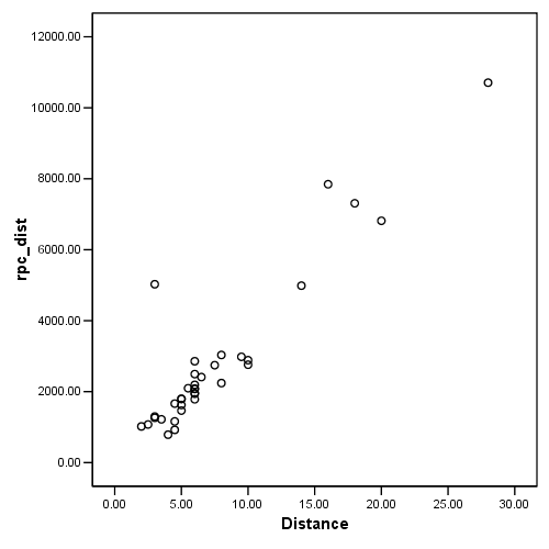
Figure 4.12(b), page 114
Note: The graph in the book is incorrect; please see errata.
graph
 /scatterplot = climb with rpc_climb.
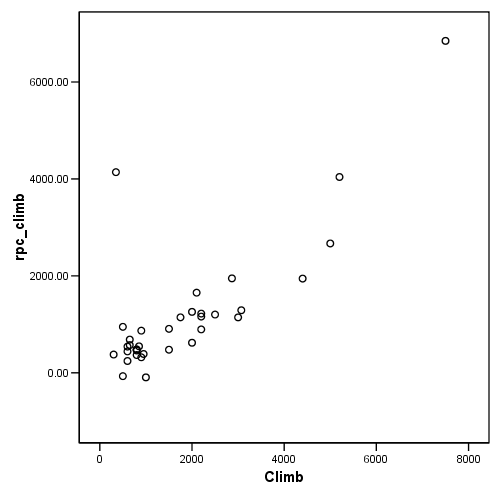
Figure 4.13, page 114. Potential-Residual plot
compute d = e/sqrt(24810082).
compute po = (pi/(1-pi)).
compute rs = ((3)/(1-pi))*(d**2/(1-d**2)).
exe.
graph
 /scatterplot = rs with po.
