Table 5.1, page 124. Salary Survey Data.
get file 'D:p124.sav'.
list.
       s        x        e        m

   13876        1        1        1
   11608        1        3        0
   18701        1        3        1
   11283        1        2        0
   11767        1        3        0
   20872        2        2        1
   11772        2        2        0
   10535        2        1        0
   12195        2        3        0
   12313        3        2        0
   14975        3        1        1
   21371        3        2        1
   19800        3        3        1
   11417        4        1        0
   20263        4        3        1
   13231        4        3        0
   12884        4        2        0
   13245        5        2        0
   13677        5        3        0
   15965        5        1        1
   12336        6        1        0
   21352        6        3        1
   13839        6        2        0
   22884        6        2        1
   16978        7        1        1
   14803        8        2        0
   17404        8        1        1
   22184        8        3        1
   13548        8        1        0
   14467       10        1        0
   15942       10        2        0
   23174       10        3        1
   23780       10        2        1
   25410       11        2        1
   14861       11        1        0
   16882       12        2        0
   24170       12        3        1
   15990       13        1        0
   26330       13        2        1
   17949       14        2        0
   25685       15        3        1
   27837       16        2        1
   18838       16        2        0
   17483       16        1        0
   19207       17        2        0
   19346       20        1        0

Number of cases read:  46    Number of cases listed:  46
Table 5.3 and Figure 5.1, page 126-127.
compute E1 = (e = 1).
compute E2 = (e = 2).
exe.
regression
 /dependent = s
 /method enter = x e1 e2 m
 /save sresid(r)
 /scatterplot (*sresid, x).
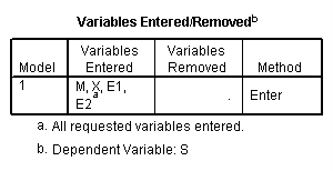
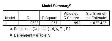
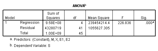
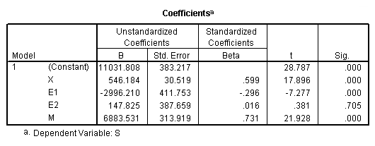
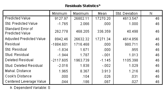
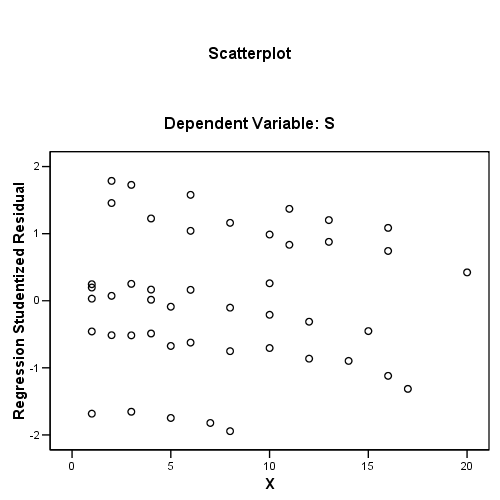
Figure 5.2, page 128. Standardized residuals versus education-management
categorical variable.
if (e = 1) & (m = 0) c = 1.
if (e = 1) & (m = 1) c = 2.
if (e = 2) & (m = 0) c = 3.
if (e = 2) & (m = 1) c = 4.
if (e = 3) & (m = 0) c = 5.
if (e = 3) & (m = 1) c = 6.
exe.
graph
 /scatterplot = c with r.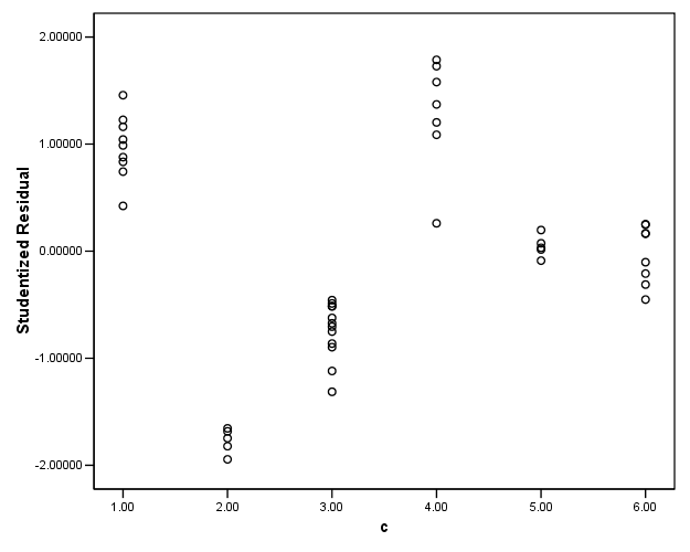
Table 5.4 and Figure 5.3, page 129. Expanded Model and standardized residuals
versus years of experience.
compute me1 = m*e1.
compute me2 = m*e2.
exe.
regression
 /dependent = s
 /method enter = x e1 e2 m me1 me2
 /scatterplot (*sresid, x).
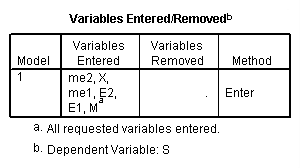
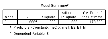
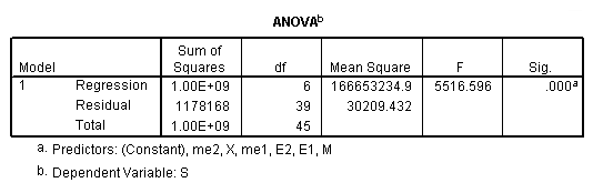
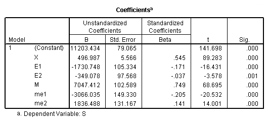
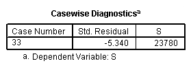
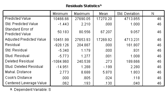
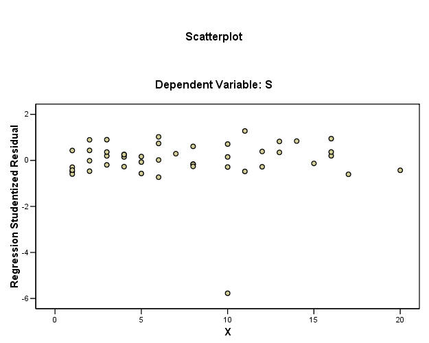
Table 5.5 and Figure 5.4, page 129-130. Expanded model (with obs. 33 deleted)
and standardized residuals versus years of experience.
compute id = $casenum.
exe.
compute filter = (id~=33).
filter by filter.
exe.
regression
 /dependent = s
 /method enter = x e1 e2 m me1 me2
 /scatterplot (*sresid, x)
 /save sresid(rs).
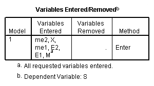
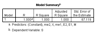
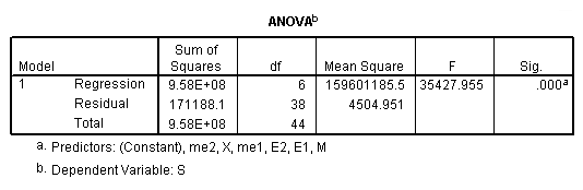
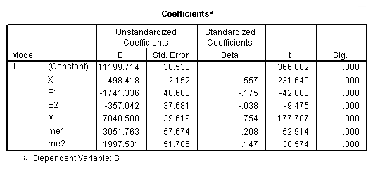
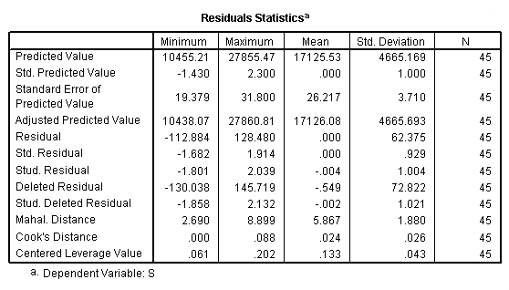
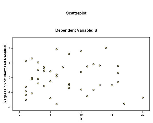
Figure 5.5, page 130. Standardized residuals versus education-management
category, (obs. 33 deleted).
graph
 /scatterplot = c with rs.
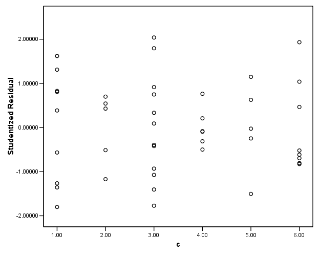
Table 5.6, page 131. Estimates of Base Salary Using the Nonadditive Model in
(5.2), (obs. 33 deleted).
glm s by e m with x
 /emmeans = tables(e*m) with(x = 0)
 /design x e m e*m.
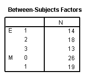
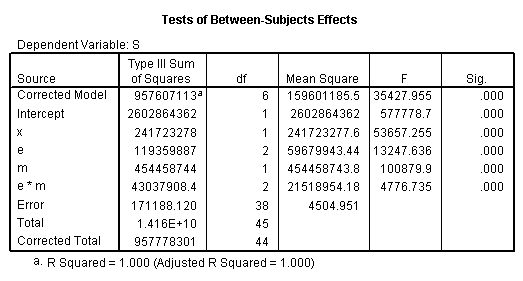
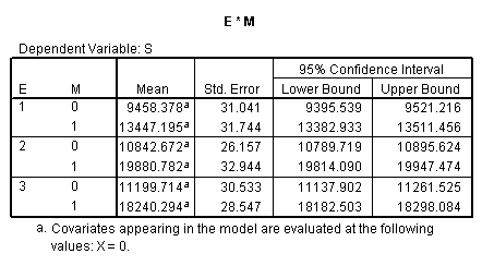
Table 5.7, page 134. Data on Preemployment Testing Program.
get file 'D:p134.sav'.
list.
     test     race     jperf

      .28        1      1.83
      .97        1      4.59
     1.25        1      2.97
     2.46        1      8.14
     2.51        1      8.00
     1.17        1      3.30
     1.78        1      7.53
     1.21        1      2.03
     1.63        1      5.00
     1.98        1      8.04
     2.36        0      3.25
     2.11        0      5.30
      .45        0      1.39
     1.76        0      4.69
     2.09        0      6.56
     1.50        0      3.00
     1.25        0      5.85
      .72        0      1.90
      .42        0      3.85
     1.53        0      2.95

Number of cases read:  20    Number of cases listed:  20
Table 5.8 and Figure 5.7, page 135.
regression
 /dependent = jperf
 /method enter = test
 /save sresid(sr)
 /scatter (*sresid, test).
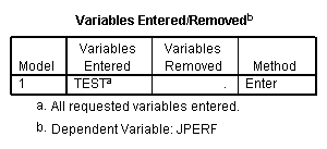
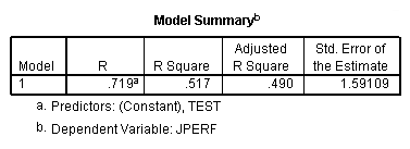
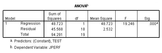
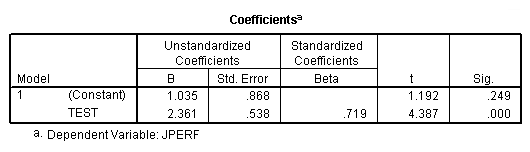
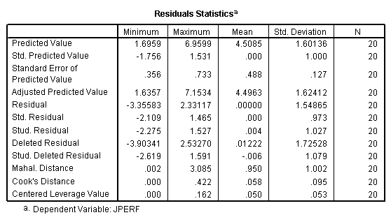
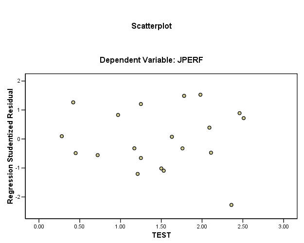
Table 5.9 and Figure 5.8, page 135.
compute rt = race*test.
exe.
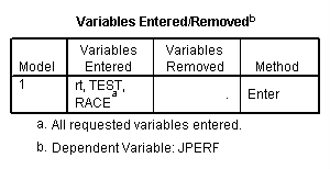
regression
 /dependent = jperf
 /method enter = test race rt
 /scatter (*sresid, test).
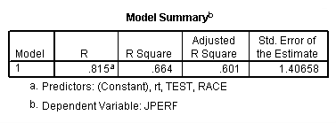
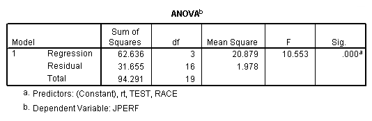
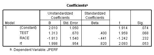
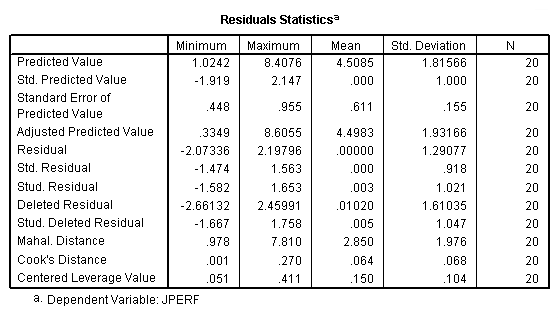
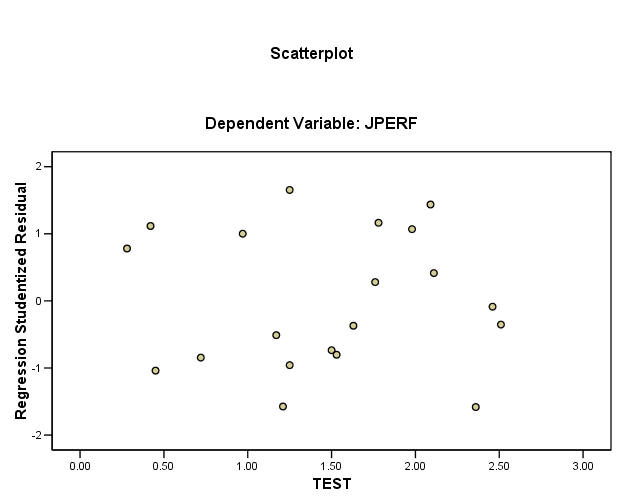
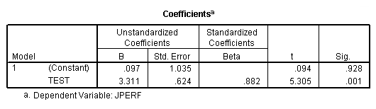
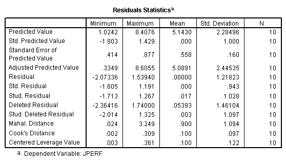
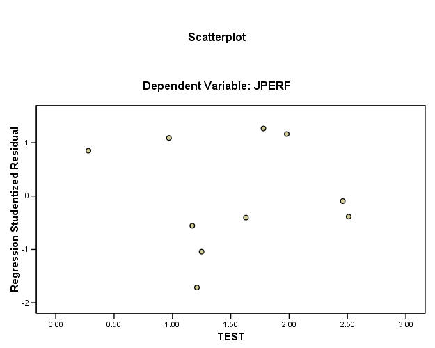
Part of Table 5.10 and Figure 5.10, page 136-137.
Use the select if command to restrict the following analysis when race
=1. The temporary command allows the restriction to last for one procedure,
after which it returns to the unrestricted data set.
temporary.
select if (race = 1).
regression
 /dependent = jperf
 /method enter = test
 /scatter (*sresid, test).
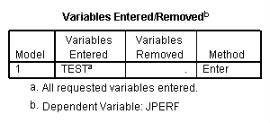
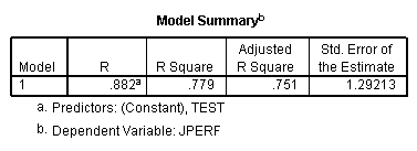
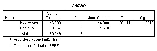
Part of Table 5.10 and Figure 5.11, page 136-137.
temporary.
select if (race = 0).
regression
 /dependent = jperf
 /method enter = test
 /scatter (*sresid, test).
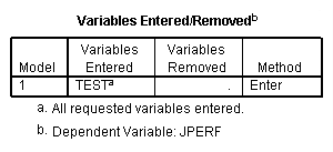
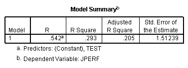
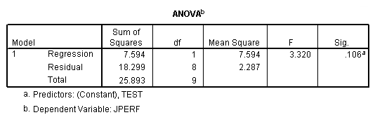
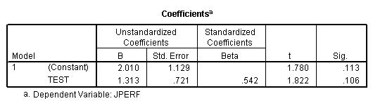
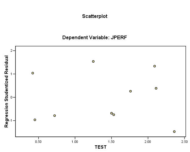
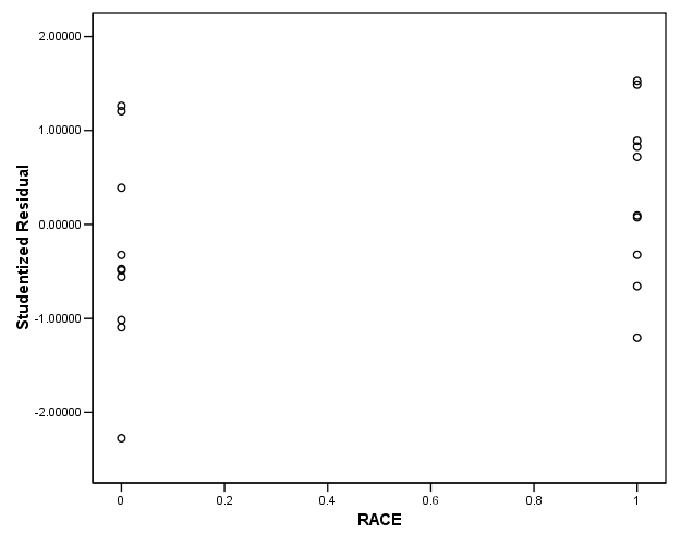
Figure 5.9, page 136.
graph
 /scatterplot = race with sr.