Table 7.3, page 189. Education Expenditure Data.
get file 'd:p189.sav'.
list.
state        y       x1       x2       x3   region

ME         235     3944      325      508        1
NH         231     4578      323      564        1
VT         270     4011      328      322        1
MA         261     5233      305      846        1
RI         300     4780      303      871        1
CT         317     5889      307      774        1
NY         387     5663      301      856        1
NJ         285     5759      310      889        1
PA         300     4894      300      715        1
OH         221     5012      324      753        2
IN         264     4908      329      649        2
IL         308     5753      320      830        2
MI         379     5439      337      738        2
WI         342     4634      328      659        2
MN         378     4921      330      664        2
IA         232     4869      318      572        2
MO         231     4672      309      701        2
ND         246     4782      333      443        2
SD         230     4296      330      446        2
NB         268     4827      318      615        2
KS         337     5057      304      661        2
DE         344     5540      328      722        3
MD         330     5331      323      766        3
VA         261     4715      317      631        3
WV         214     3828      310      390        3
NC         245     4120      321      450        3
SC         233     3817      342      476        3
GA         250     4243      339      603        3
FL         243     4647      287      805        3
KY         216     3967      325      523        3
TN         212     3946      315      588        3
AL         208     3724      332      584        3
MS         215     3448      358      445        3
AR         221     3680      320      500        3
LA         244     3825      355      661        3
OK         234     4189      306      680        3
TX         269     4336      335      797        3
MT         302     4418      335      534        4
ID         268     4323      344      541        4
WY         323     4813      331      605        4
CO         304     5046      324      785        4
NM         317     3764      366      698        4
AZ         332     4504      340      796        4
UT         315     4005      378      804        4
NV         291     5560      330      809        4
WA         312     4989      313      726        4
OR         316     4697      305      671        4
CA         332     5438      307      909        4
AK         546     5613      386      484        4
HI         311     5309      333      831        4
Number of cases read: 50 Number of cases listed: 50
Table 7.4 and Figure 7.3, 7.5-7.7, page 191.
regression
 /dependent = y
 /method enter = x1 x2 x3
 /scatter (*sresid, *pred) (*sresid, x1) (*sresid, x2) (*sresid, x3)
 /save sresid(sr).
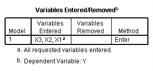
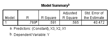
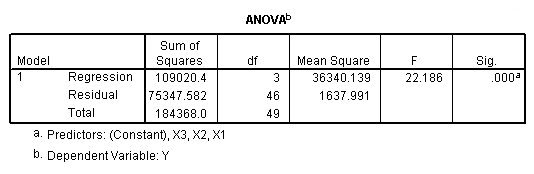
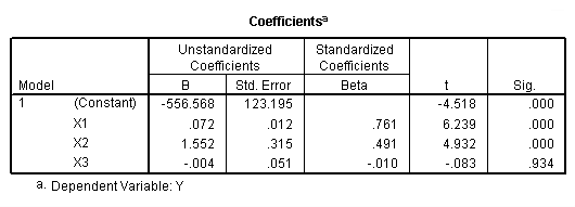
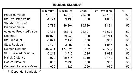
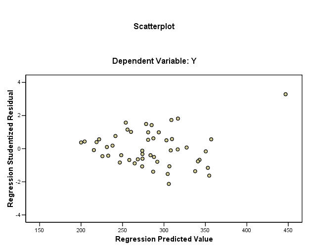
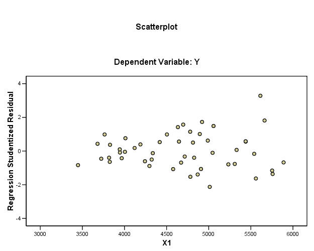
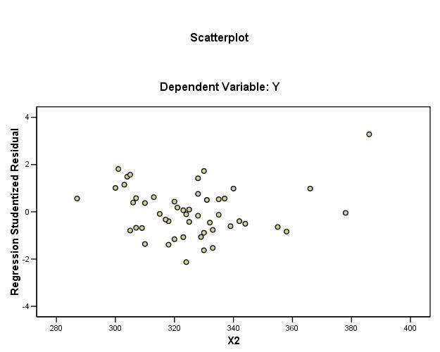
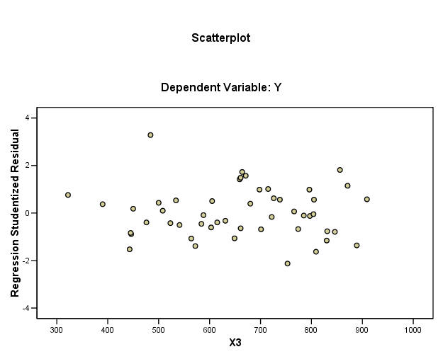
Figure 7.4, page 191.
graph
 /scatterplot = region with sr.
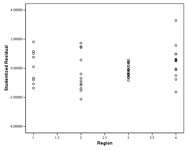
Table 7.5 and Figure 7.8, page 194-195. Alaska omitted.
select if (state ~= "AK").
regression
 /dependent = y
 /method enter = x1 x2 x3
 /scatter (*sresid, *pred)
 /save sresid(sr_ak).
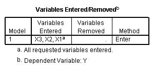
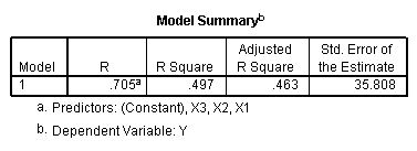
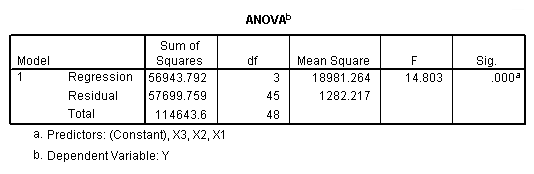
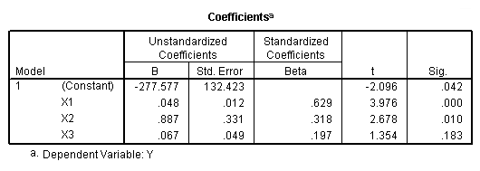
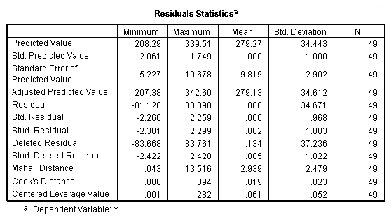
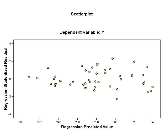
Figure 7.9, page 194.
graph
 /scatterplot = region with sr_ak.
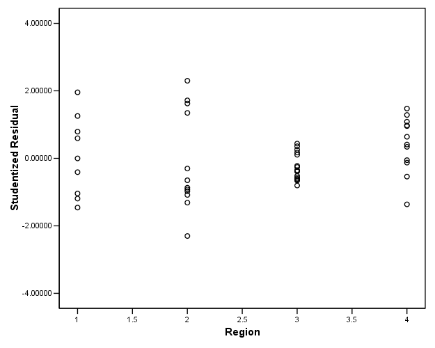
Table 7.6, page 195. Weights cj for Weighted Least Squares.
Calculation of weights is from the residuals from the regression.
regression /dependent = y /method enter = x1 x2 x3 /save resid(r).[output omitted]
compute r2 = r**2.
compute const = 1.
exe.

aggregate outfile "e:tempag1.sav"
 /break =region
 /s2 = mean(r2).
aggregate outfile "e:tempag2.sav"
 /break =const
 /r2mean = mean(r2).
match files file = *
 /table ="e:tempag1.sav"
 /by region.
match files file = *
/table = "e:tempag2.sav"
/by const.
exe.

compute c = sqrt(s2/r2mean).
exe.

temporary.
split file by region.
descriptives var = c r2
 /stats = mean.
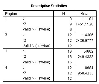
Table 7.7, page 195. WLS coefficients for the education data (Alaska
omitted).
compute weight = c**-2.
exe.
regression
 /regwgt = weight
 /dependent = y
 /method enter = x1 x2 x3
 /save resid(wlsr) pred(wlsp).
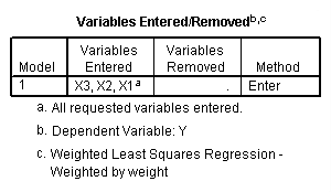
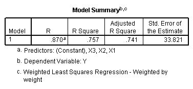
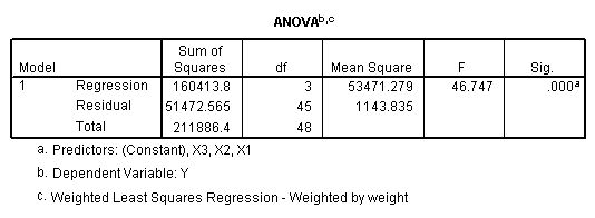
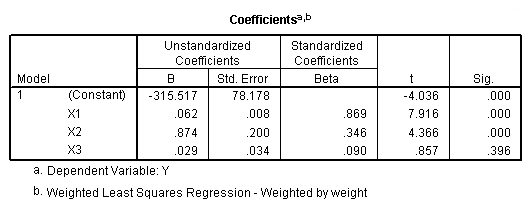
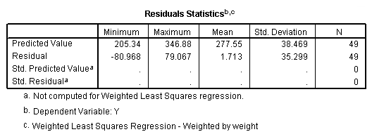
Figure 7.10, page 196. Standardized residuals versus fitted values of for WLS
solution.
NOTE 1: The predicted values and residuals need to be adjusted to account for
the weighting.
NOTE 2: Used unstandardized residuals, so the scaling is off from the text.
compute wp = wlsp/c.
compute wr = wlsr/c.
exe.
graph
 /scatterplot = wp with wr.
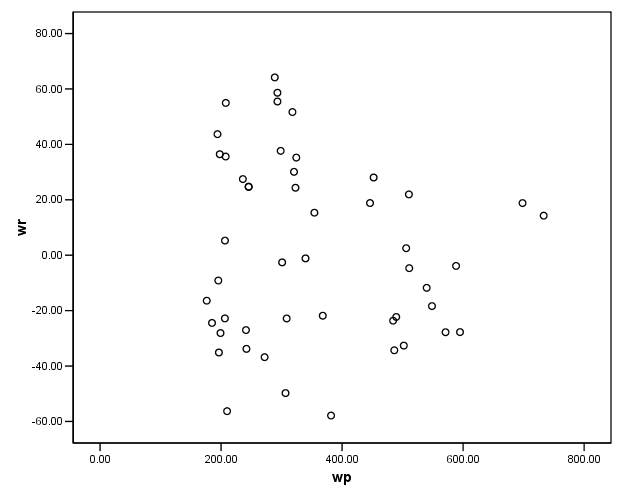
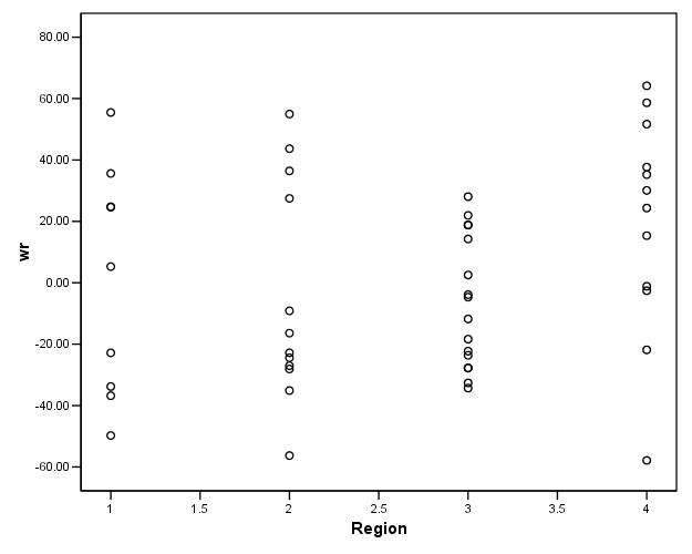
Figure 7.11, page 196. Standardized residuals by geographic region for WLS
solution.
graph
 /scatterplot = region with wr.