Table 8.1, page 203. Consumer Expenditure and Money Stock.
get file 'd:p203.sav'.
list.
    year  quarter  expendit     stock

    1952        1    214.60    159.30
    1952        2    217.70    161.20
    1952        3    219.60    162.80
    1952        4    227.20    164.60
    1953        1    230.90    165.90
    1953        2    233.30    167.90
    1953        3    234.10    168.30
    1953        4    232.30    169.70
    1954        1    233.70    170.50
    1954        2    236.50    171.60
    1954        3    238.70    173.90
    1954        4    243.20    176.10
    1955        1    249.40    178.00
    1955        2    254.30    179.10
    1955        3    260.90    180.20
    1955        4    263.30    181.20
    1956        1    265.60    181.60
    1956        2    268.20    182.50
    1956        3    270.40    183.30
    1956        4    275.60    184.30


Number of cases read:  20    Number of cases listed:  20
Table 8.2, page 203. Consumer Expenditure is Regressed on Money Stock.
regression
 /dependent = expendit
 /method enter = stock
 /save sresid(sr).
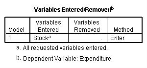
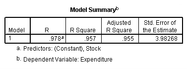
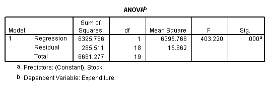
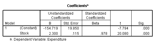
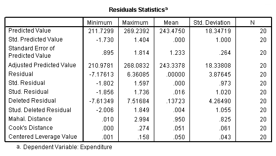
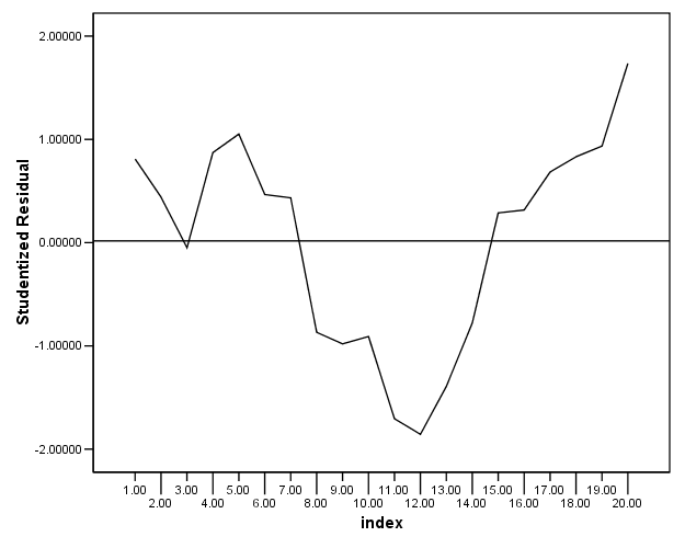
Figure 8.1, page 204. Index plot of the standardized residuals.
compute index = $casenum.
exe.
tsplot variable = sr
 /id = index
 /format reference.
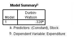
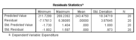
Durbin Watson Statistic, page 205.
regression
 /statistics outs
 /dependent = expendit
 /method enter = stock
 /residual durbin.
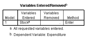
Section 8.4 and 8.5, page 206-209.
The areg command that handles autocorrelation is not available on base
SPSS.
Table 8.4, page 211.
get file 'd:p211.sav'.
list.

        h         p         d

      .09      2.20       .04
      .09      2.22       .03
      .10      2.24       .04
      .10      2.27       .04
      .10      2.28       .04
      .10      2.29       .04
      .11      2.29       .05
      .11      2.29       .05
      .11      2.30       .05
      .11      2.30       .05
      .11      2.30       .05
      .11      2.34       .06
      .11      2.39       .05
      .12      2.43       .05
      .12      2.48       .05
      .12      2.53       .06
      .12      2.58       .06
      .12      2.61       .06
      .12      2.63       .05
      .13      2.66       .06
      .13      2.68       .07
      .13      2.71       .06
      .13      2.74       .06
      .14      2.77       .07
      .14      2.79       .07


Number of cases read:  25    Number of cases listed:  25
Table 8.5, page 212. Regression on Housing Starts (H) versus Population (P).
regression
 /dependent = h
 /method enter = p
 /save sresid(sr).
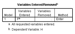
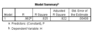
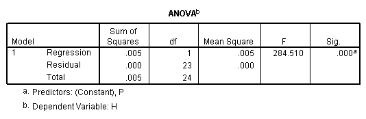
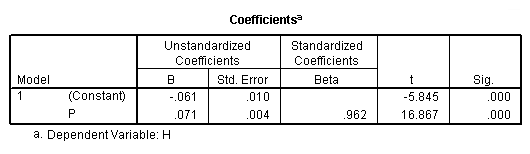
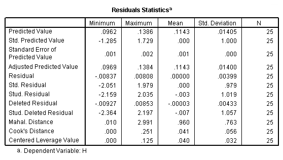
Figure 8.3, page 212. Index plot of residuals from table 8.5.
compute index = $casenum.
exe.
tsplot variable = sr
 /id=index
 /format reference.
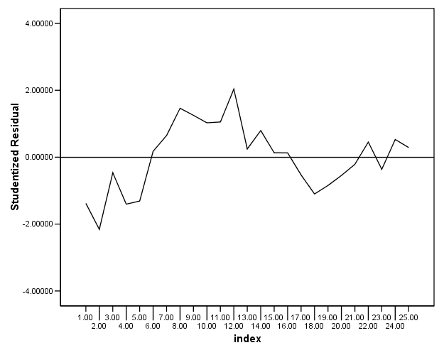
Table 8.6, page 213.
regression
 /dependent = h
 /method enter = p d
 /save sresid(sr2).
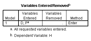
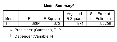
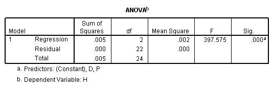
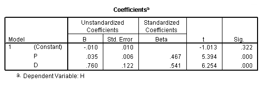
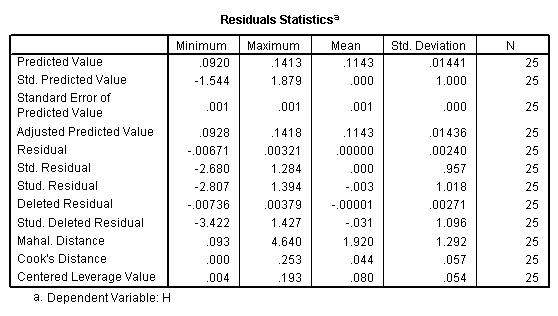
Figure 8.4, page 213. Index plot of residuals from table 8.6.
tsplot variable = sr2
 /id=index
 /format reference.
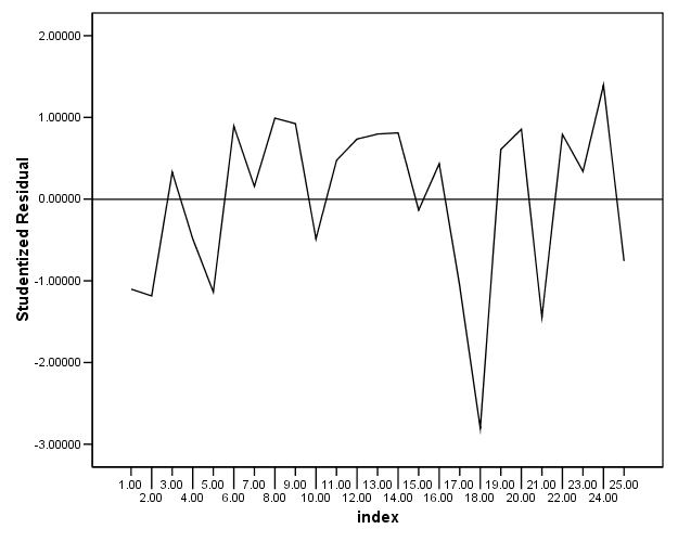
For the equation on top of page 214, see the standardized coefficients column
from the regression from Table 8.6.
Table 8.7, page 215. Ski Sales versus PDI.
get file 'd:p217.sav'.
regression
 /dependent = sales
 /method enter = pdi
 /residual durbin
 /save sres /save sresid(sr).
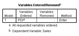
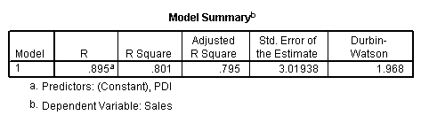
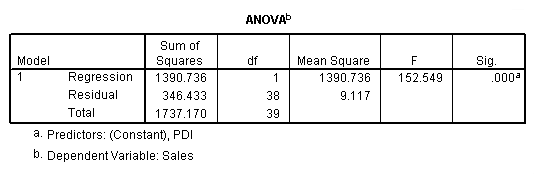
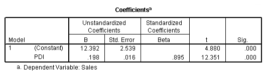
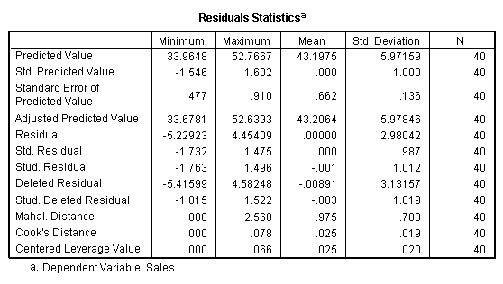
Figure 8.5, page 215. Index plot of residuals differentiating between season.
compute index = $casenum.
exe.
formats sr (f8.2) index (f2.0).
GGRAPH
  /GRAPHDATASET NAME="GraphDataset" VARIABLES= sr index season
  /GRAPHSPEC SOURCE=INLINE .
BEGIN GPL
SOURCE: s=userSource( id( "GraphDataset" ) )
DATA: sr=col( source(s), name( "sr" ) )
DATA: index=col( source(s), name( "index" ) )
DATA: season = col( source(s), name( "season" ), unit.category() )
GUIDE: axis( dim( 1 ), label( "index" ) )
GUIDE: axis( dim( 2 ), label( "Residuals" ), start(0.0), delta(.75) )
SCALE: linear( dim( 1 ) )
SCALE: linear( dim( 2 ), min(-1.50), max(1.50) )
ELEMENT: point( position( ( index * sr ) ), shape( season ) )
END GPL.
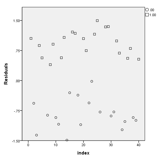
Table 8.8, page 217. Disposable Income and Ski Sales, and Seasonal variables
for years 1964-1973.
list.

quarter     sales      pdi   season          sr    index

Q1/64       37.00      109        1     1.05164     1.00
Q2/64       33.50      115        0     -.56792     2.00
Q3/64       30.80      113        0    -1.36335     3.00
Q4/64       37.90      116        1      .87534     4.00
Q1/65       37.40      118        1      .56648     5.00
Q2/65       31.60      120        0    -1.55216     6.00
Q3/65       34.00      122        0     -.86544     7.00
Q4/65       38.10      124        1      .39704     8.00
Q1/66       40.00      126        1      .90737     9.00
Q2/66       35.00      128        0     -.92432    10.00
Q3/66       34.90      130        0    -1.09078    11.00
Q4/66       40.20      132        1      .56917    12.00
Q1/67       41.90      133        1     1.07638    13.00
Q2/67       34.70      135        0    -1.48856    14.00
Q3/67       38.80      138        0     -.30469    15.00
Q4/67       43.70      140        1     1.21173    16.00
Q1/68       44.20      143        1     1.17872    17.00
Q2/68       40.40      147        0     -.36450    18.00
Q3/68       38.40      148        0    -1.10224    19.00
Q4/68       45.40      151        1     1.04776    20.00
Q1/69       44.90      153        1      .74703    21.00
Q2/69       41.60      156        0     -.55906    22.00
Q3/69       44.00      160        0     -.01960    23.00
Q4/69       48.10      163        1     1.15735    24.00
Q1/70       49.70      166        1     1.49628    25.00
Q2/70       43.90      171        0     -.78603    26.00
Q3/70       41.60      174        0    -1.76254    27.00
Q4/70       51.00      175        1     1.33981    28.00
Q1/71       52.00      180        1     1.34764    29.00
Q2/71       46.20      184        0     -.88522    30.00
Q3/71       47.10      187        0     -.78336    31.00
Q4/71       52.70      189        1      .98941    32.00
Q1/72       52.20      191        1      .68540    33.00
Q2/72       47.00      193        0    -1.22901    34.00
Q3/72       47.80      194        0    -1.02404    35.00
Q4/72       52.80      196        1      .55547    36.00
Q1/73       54.10      199        1      .80119    37.00
Q2/73       49.50      201        0     -.92441    38.00
Q3/73       49.50      202        0     -.99426    39.00
Q4/73       54.30      204        1      .53260    40.00


Number of cases read:  40    Number of cases listed:  40
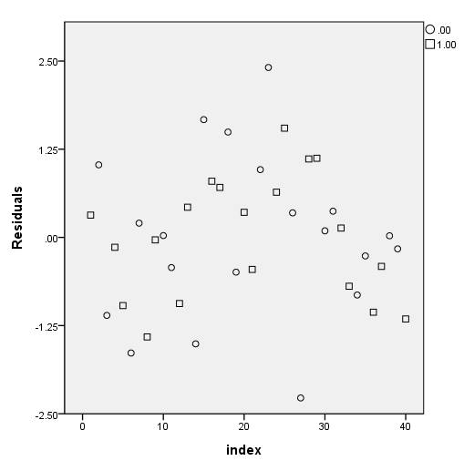
Table 8.9, page 217. Ski Sales versus PDI and Seasonal Variables.
regression
 /dependent = sales
 /method enter = pdi season
 /residual durbin
 /save sresid(sr2).
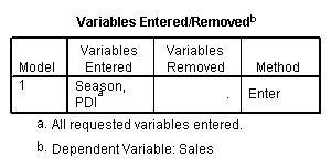
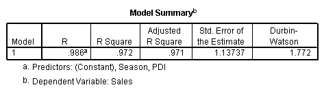
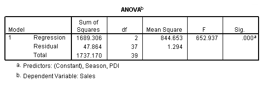
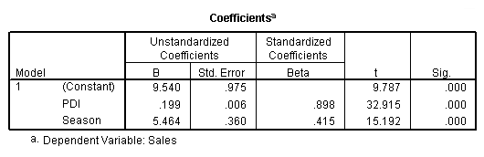
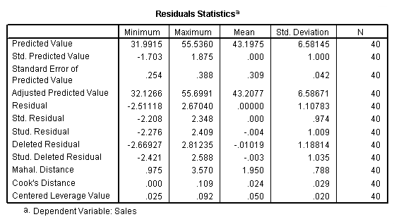
Figure 8.7, page 218.
formats sr2 (f8.2).
GGRAPH
  /GRAPHDATASET NAME="GraphDataset" VARIABLES= sr2 index season
  /GRAPHSPEC SOURCE=INLINE .
BEGIN GPL
SOURCE: s=userSource( id( "GraphDataset" ) )
DATA: sr2=col( source(s), name( "sr2" ) )
DATA: index=col( source(s), name( "index" ) )
DATA: season = col( source(s), name( "season" ), unit.category() )
GUIDE: axis( dim( 1 ), label( "index" ), start(0.0), delta(10) )
GUIDE: axis( dim( 2 ), label( "Residuals" ), start(0.0), delta(1.25) )
SCALE: linear( dim( 1 ), min(0), max(40) )
SCALE: linear( dim( 2 ), min(-2.50), max(2.50) )
ELEMENT: point( position( ( index * sr2 ) ), shape( season ) )
END GPL.