Table 9.1, page 228. Equal Educational Opportunity (EEO) Data (First 10
Observations).
get file 'd:p228.sav'.
list
 /cases = 10 .
     achv       fam      peer    school

     -.43       .61       .04       .17
      .80       .79       .48       .53
     -.92      -.83      -.62      -.79
    -2.19     -1.25     -1.22     -1.04
    -2.85       .17      -.19       .14
     -.66       .20       .13       .27
     2.64       .24      -.09       .05
     2.36       .59       .22       .52
     -.91      -.62      -.49      -.63
      .59       .99       .62       .93

Number of cases read:  10    Number of cases listed:  10
Table 9.3 and Figure 9.1, page 229.
regression
 /dependent = achv
 /method enter = fam peer school
 /scatterplot (*sresid, *pred).
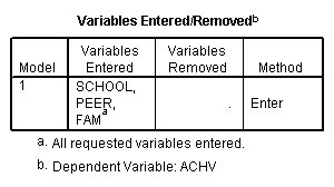
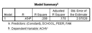
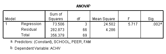
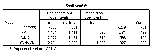
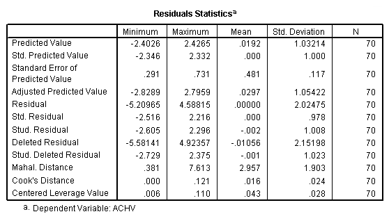
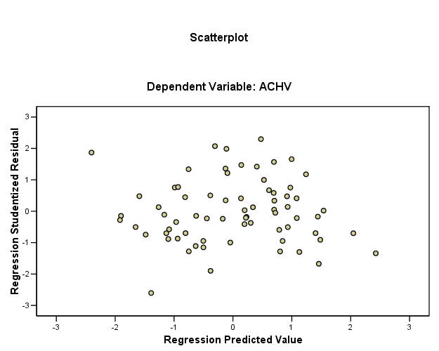
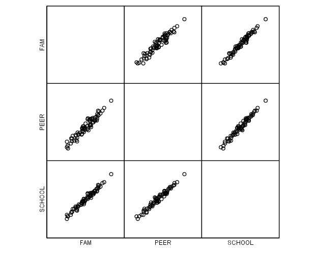
Figure 9.2, page 231. Pairwise scatterplots and correlations of the three
predictors variables FAM, PEER and SCHOOL.
graph
 /scatterplot(matrix) = fam peer school.
correlations variables = fam peer school.
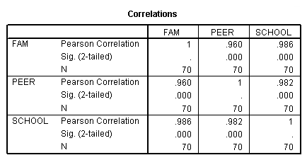
Table 9.12, page 242. EEO Data VIF.
regression
 /statistics tol
 /dependent = achv
 /method enter = fam peer school.
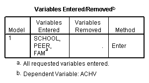
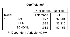
Table 9.5, page 233. Data on French Economy.
get file 'd:p233.sav'.
list.
    year    import    doprod     stock    consum

      49     15.90    149.30      4.20    108.10
      50     16.40    161.20      4.10    114.80
      51     19.00    171.50      3.10    123.20
      52     19.10    175.50      3.10    126.90
      53     18.80    180.80      1.10    132.10
      54     20.40    190.70      2.20    137.70
      55     22.70    202.10      2.10    146.00
      56     26.50    212.40      5.60    154.10
      57     28.10    226.10      5.00    162.30
      58     27.60    231.90      5.10    164.30
      59     26.30    239.00       .70    167.60
      60     31.10    258.00      5.60    176.80
      61     33.30    269.80      3.90    186.60
      62     37.00    288.40      3.10    199.70
      63     43.30    304.50      4.60    213.90
      64     49.00    323.40      7.00    223.80
      65     50.30    336.80      1.20    232.00
      66     56.60    353.90      4.50    242.90

Number of cases read:  18    Number of cases listed:  18
Table 9.6, page 234. Import Data (1949-1966): Regression Results.
regression
 /dependent = import
 /method enter = doprod stock consum
 /save sresid(sr).
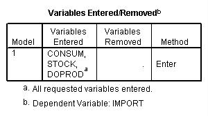
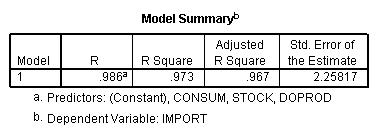
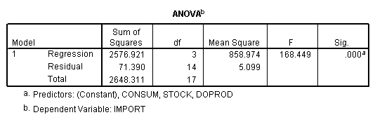
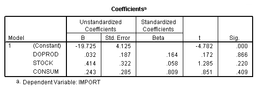
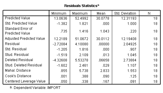
Figure 9.3, page 234. Index plot (1949-1966).
compute index = $casenum.
tsplot variable = sr
 /id=index
 /format reference.
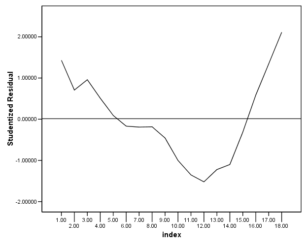
Table 9.7, page 235. Import Data (1949-1959): Regression Results.
compute filter = (year <= 59).
filter by filter.
exe.
regression
 /dependent = import
 /method enter = doprod stock consum
 /save sresid(sr2).
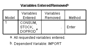
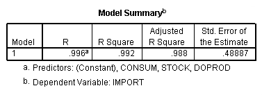
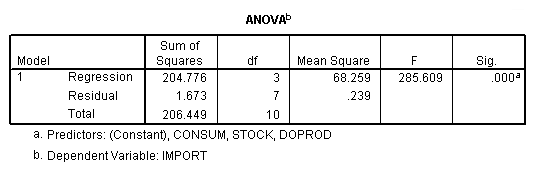
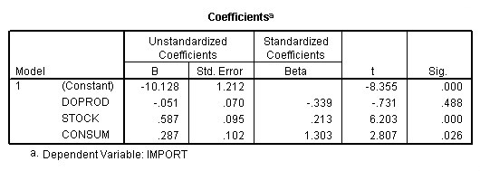
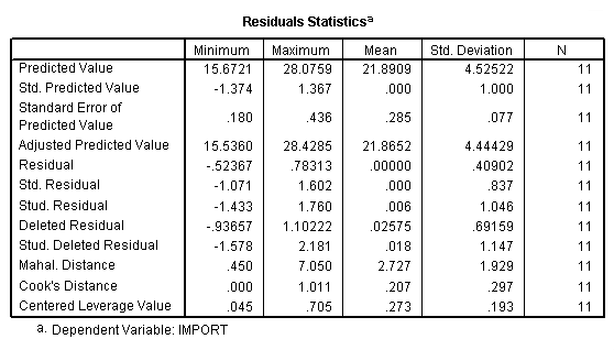
Figure 9.4, page 234. Index plot (1949-1959).
compute index = $casenum.
tsplot variable = sr2
 /id=index
 /format reference.
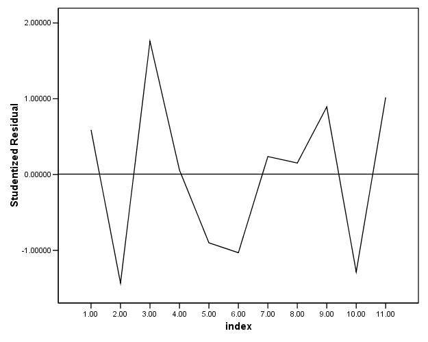
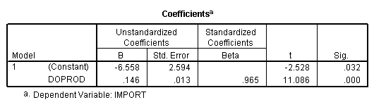
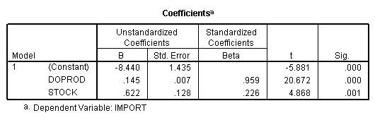
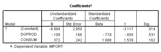
Table 9.8, page 237. Import Data (1949-1959): Regression Coefficients for All
Possible Regressions.
regression
 /statistics coef
 /dependent = import
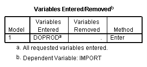
 /method enter = doprod.
regression
 /statistics coef
 /dependent = import
 /method enter = stock.
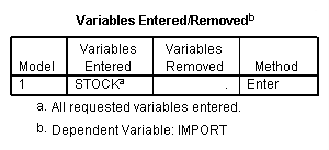
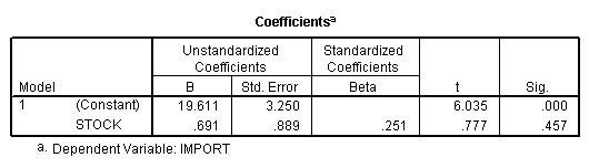
regression
 /statistics coef
 /dependent = import
 /method enter = consum.
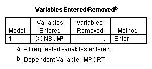
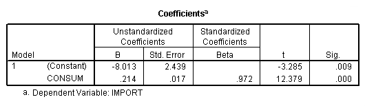
regression
 /statistics coef
 /dependent = import
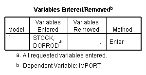
 /method enter = doprod stock.
regression
 /statistics coef
 /dependent = import
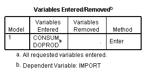
 /method enter = doprod consum.
regression
 /statistics coef
 /dependent = import
 /method enter = stock consum.
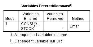
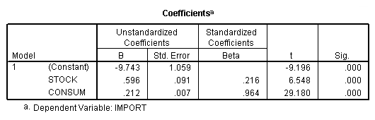
regression
 /statistics coef
 /dependent = import
 /method enter = doprod stock consum.
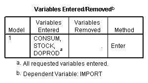
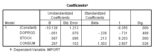
Table 9.12, page 242. IMPORT Data VIF .
NOTE: VIF was conducted on full IMPORT data set, not reduced (1949-1959).
use all.
regression
 /statistics tol
 /dependent = import
 /method enter = doprod stock consum.
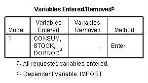
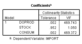
Table 9.9, page 238. Annual Data on Advertising, Promotions, Sales Expenses,
and Sales.
get file 'd:p238.sav'.
list.

      s_t       a_t       p_t       e_t      a_t1      p_t1

    20.11      1.99      1.00       .30      2.02       .00
    15.10      1.94       .00       .30      1.99      1.00
    18.68      2.20       .80       .35      1.94       .00
    16.05      2.00       .00       .35      2.20       .80
    21.30      1.69      1.30       .30      2.00       .00
    17.85      1.74       .30       .32      1.69      1.30
    18.88      2.07      1.00       .31      1.74       .30
    21.27      1.02      1.00       .41      2.07      1.00
    20.48      2.02       .90       .45      1.02      1.00
    20.54      1.06      1.00       .45      2.02       .90
    26.18      1.46      1.50       .50      1.06      1.00
    21.72      1.88       .00       .60      1.46      1.50
    28.70      2.27       .80       .65      1.88       .00
    25.84      1.11      1.00       .65      2.27       .80
    29.32      1.77      1.20       .65      1.11      1.00
    24.19       .96      1.00       .65      1.77      1.20
    26.59      1.99      1.00       .62       .96      1.00
    22.24      1.97       .00       .60      1.99      1.00
    24.80      2.27       .70       .60      1.97       .00
    21.19      1.98       .10       .61      2.27       .70
    26.03      2.10      1.00       .60      1.98       .10
    27.39      1.07      1.00       .58      2.10      1.00

Number of cases read:  22    Number of cases listed:  22
Table 9.10 and Figure 9.5, page 239.
regression
 /dependent = s_t
 /method enter = a_t p_t e_t a_t1 p_t1
 /scatterplot (*sresid, *pred)
 /save sresid(sr).
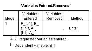
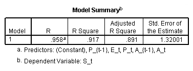
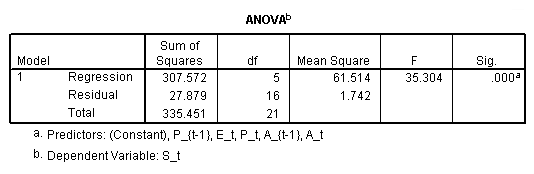
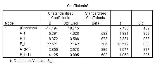
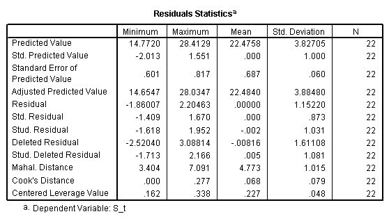
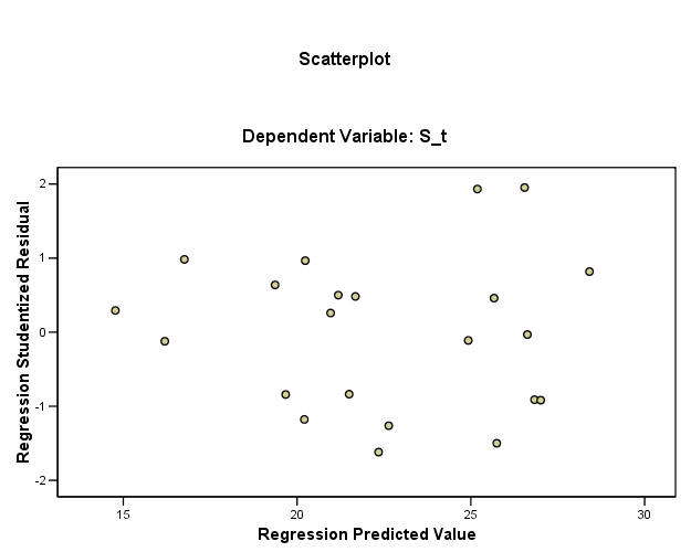
Table 9.11, page 239. Pairwise correlation coefficients for the advertising
data.
correlations variables = a_t p_t e_t a_t1 p_t1.
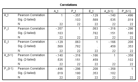
Figure 9.6, page 240. Index plot.
compute index = $casenum.
exe.
tsplot variable = sr
 /id=index
 /format reference.
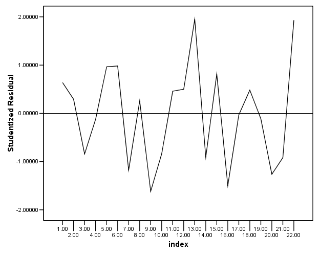
Table 9.12, page 242. Advertising Data VIF.
NOTE: VIF for a_t, a_t1 and p_t1 do not match the text.
regression
 /statistics tol
 /dependent = s_t
 /method enter = a_t p_t e_t a_t1 p_t1.
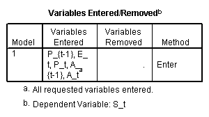
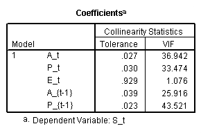
Table 9.13, page 247 .
get file 'd:p233.sav'.
select if (year <= 59).
exe.
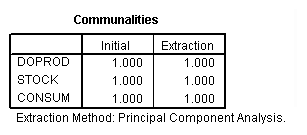
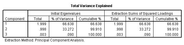
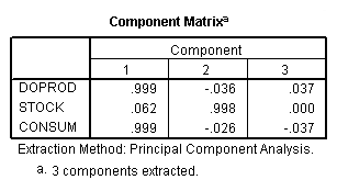
factor variables = doprod stock consum
 /criteria factors(3) iterate(25)
 /extraction pc
 /rotation norate
 /save reg( 3, fs).
list variables year fs1 fs2 fs3.
    year         fs1         fs2         fs3

      49    -1.50355      .63925      .39948
      50    -1.14500      .55605     1.37089
      51     -.78871     -.07305      .41891
      52     -.63250     -.08245     -.20845
      53     -.45562    -1.30789    -1.39922
      54     -.13463     -.65976     -.51187
      55      .25434     -.74436     -.82471
      56      .68731     1.35531    -1.21184
      57     1.10284      .96494     -.45445
      58     1.24972     1.01616      .86726
      59     1.36578    -1.66420     1.55401

Number of cases read:  11    Number of cases listed:  11
NOTE: SPSS gives factor scores, whereas in SAS or STATA you’d can either get
principal component or factor scores. There is a direct linear transformation
between the two scoring methods, for this example they are,
princ1score = factor1score*1.41397
princ2score = factor2score*0.99908
princ3score = factor3score*0.051874
Importantly, the standardized beta coefficients in the regression model for the
two scoring methods are the same. The analysis in the rest of this chapter will
be done using factors scores, therefore the results won’t match the book.
Table 9.14, page 250 and Figure 9.8, page 251.
compute newvar = doprod + consum.
exe.
regression
 /dependent = import
 /method enter = stock newvar
 /save sresid(sr)
 /scatterplot (*sresid, *pred).
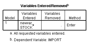
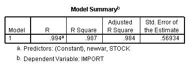
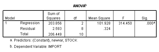
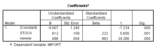
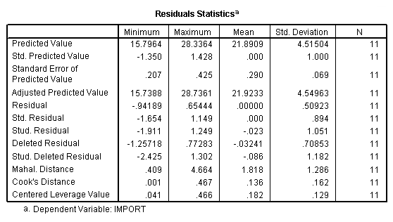
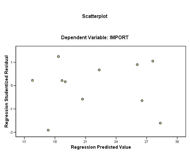
Figure 9.7, page 251. Index plot.
compute index = $casenum.
exe.
tsplot variable = sr
 /id=index
 /format reference.
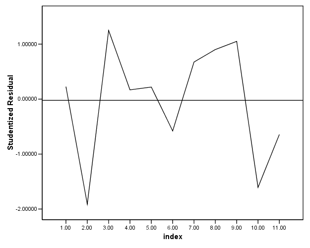
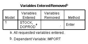
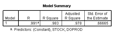
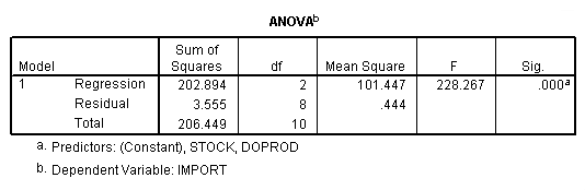
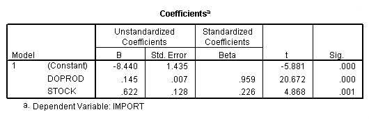
Table 9.15, page 253. Regression results when fitting model (9.26) to the
Import Data (1949-1959).
regression
/dependent = import
/method enter = doprod stock.
Eigenvectors for equation (9.27), page 253.
NOTE, we are using factor scores rather than principal component scores.
get file 'd:p238.sav'.
factor variables = a_t p_t e_t a_t1 p_t1
 /criteria factors(5) iterate(25)
 /extraction pc
 /rotation norate
 /save reg( 5, fs).
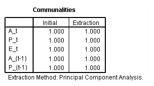
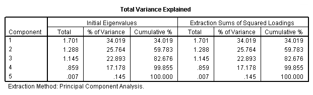
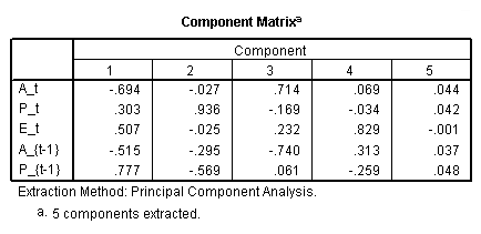
Table 9.16, page 256. Standardized regression results obtained from fitting
the model in (9.29).
regression
 /dependent = s_t
 /method enter = a_t p_t e_t a_t1 p_t1.
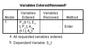
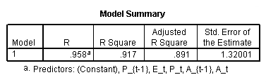
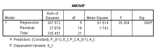
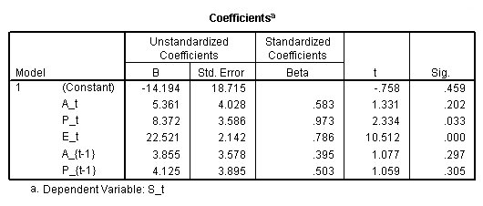
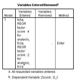
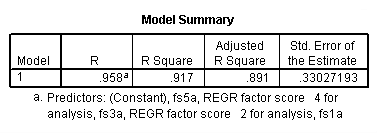
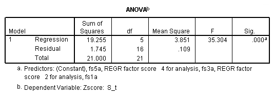
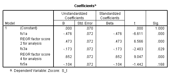
Table 9.17, page 257. Regression results obtained from fitting the model in
(9.31).
NOTE 1: The standardized regression coefficients from the factor scores match those from
the principal component scores. The PC’s found by SAS were the additive inverses
of those in the book. For a quick fix to get them to be exactly the same just
transform them by -1.
NOTE 2: To match the book, fs1 fs3 and fs5 need to multiplied by -1.
NOTE 3: The dependent variable was transformed to its standardized value with
the descriptive command using the save subcommand.
compute fs1a = -fs1.
compute fs3a = -fs3.
compute fs5a = -fs5.
exe.
descriptives variables = s_t
 /save.
[output omitted]
regression
 /dependent = zs_t
 /method enter = fs1a fs2 fs3a fs4 fs5a.