Page 271 Figure 12.1 Logistic function for the depression data set
NOTE: We were unable to reproduce this graph.
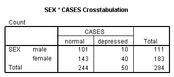
Page 273 Table 12.1 Classification of individuals by depression level and sex
get file 'c:pma5depress.sav'.
crosstabs
 /tables = sex by cases.
Page 274 Odds ratios and coefficients
compute sex1 = sex - 1.
logistic regression cases with sex1.
<some output omitted>

Page 275 The coefficients at the bottom of the page
logistic regression cases
 /method = enter age income.
<some output omitted>

Page 276 These numbers are obtained from the output from page 275.
Page 278 Table at the top of the page
compute duminc = 1.
if income >=10 duminc = 0.
compute dumemp = 0.
if employ = 2 dumemp = 1.
if employ = 3 dumemp = 1.
if employ = 7 dumemp = $sysmis.
exe.
logistic cases with duminc dumemp.
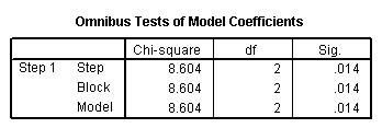

<some output omitted>
Page 279 Table in the middle of the page
compute dincemp = duminc*dumemp.
logistic cases with duminc dumemp dincemp.
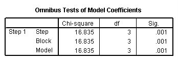
<some output omitted>
Page 280 bottom of the page
NOTE: The likelihood ratio chi-square values needed are given in the output for the two models shown above: 16.83-8.6 = 8.23.
Page 287 middle of the page
compute age0 = 0.
if age < 28 age0 = 1.
compute age1 = 0.
if age >=28 and age <= 42 age1 = 1.
compute age2 = 0.
if age >=43 and age <= 58 age2 = 1.
compute age3 = 0.
if age >=59 and age <= 89 age3 = 1.
exe.
logistic cases with age1 age2 age3 income sex.
<some output omitted>
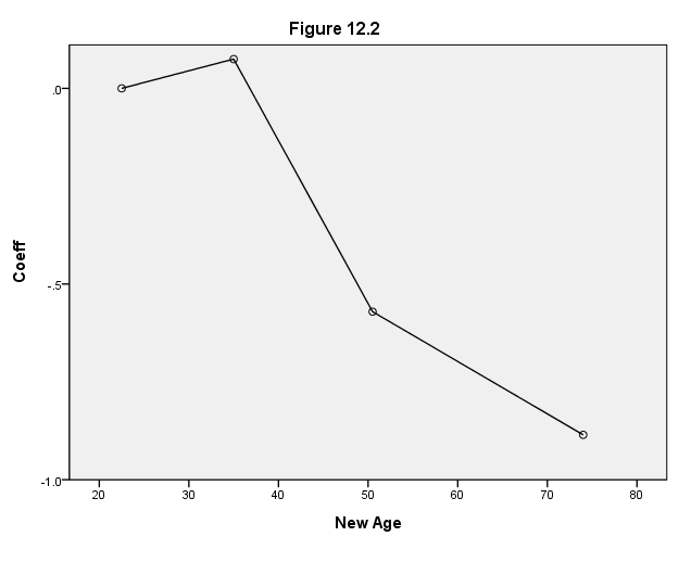
Page 289 Figure 12.2 Estimated coefficients for age quartiles by midpoint of the quartile
data list list
 /coef newage.
begin data.
0 22.5
.0747259 35
-.5706276 50.5
-.8853103 74
end data.
formats coef (f3.1) newage (f2.0).
GGRAPH
  /GRAPHDATASET NAME="GraphDataset" VARIABLES= coef newage
  /GRAPHSPEC SOURCE=INLINE .
BEGIN GPL
SOURCE: s=userSource( id( "GraphDataset" ) )
DATA: coef=col( source(s), name( "coef" ) )
DATA: newage=col( source(s), name( "newage" ) )
GUIDE: text.title( label( "Figure 12.2" ) )
GUIDE: axis( dim( 1 ), label( "New Age" ) )
GUIDE: axis( dim( 2 ), label( "Coeff" ), delta(.5) )
SCALE: linear(dim(2), min(-1), max(0))
ELEMENT: point( position( newage * coef ) )
ELEMENT: line( position( newage * coef ) )
END GPL.
Page 291 Figure 12.3 Delta beta measures to assess the influence of individual patterns on estimated coefficients
NOTE: We have skipped this graph for now.
Page 292 Table 12.2 Percent change in estimated parameters when including and excluding influential patterns
NOTE: We have skipped this graph for now.
Page 293 Table 12.3 Estimated probability of being a case (p-hat) for five influential observations
NOTE: We have skipped this graph for now.
Page 294 Figure 12.4 Delta chi-square measure to assess influence of pattern on overall fit with symbol size proportional to delta beta
NOTE: We have skipped this graph for now.
Page 296 Figure 12.5 Percentage of individuals correctly classified by logistic regression
NOTE: We have skipped this graph for now.
Page 297 Figure 12.6 ROC curve from logistic regression for the depression data set
NOTE: We have skipped this graph for now.
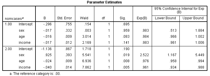
Page 300 Table 12.4 Estimated coefficients from nominal logistic regression
compute nomcases = 0.
execute.
if (cesd LE 9) nomcases = 0.
if ((cesd GE 10) AND (cesd LE 15)) nomcases = 1.
if (cesd GE 16) nomcases = 2.
execute.

nomreg nomcases (base = 0) with sex age income
  /print = lrt cps mfi parameter summary.
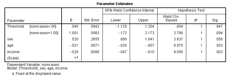
Page 303 Table 12.5 Estimated coefficients from ordinal logistic regression
GENLIN nomcases (ORDER=ASCENDING) WITH sex age income
  /MODEL sex age income
 DISTRIBUTION=MULTINOMIAL LINK=CUMLOGIT
  /PRINT CPS DESCRIPTIVES MODELINFO FIT SUMMARY SOLUTION.
