Version info: Code for this page was tested in SPSS 20.
For this chapter, you will need to use the syntax provided in Appendix A to access the School and Mice datasets.
Figure 18.2, page 466
DATASET ACTIVATE School.
* figure 18.2, page 466.
compute sch = numeric(school, F4.0).
aggregate
/outfile = * mode = addvariables
/break = sch
/med = median(math).

sort cases by med.
compute index1 = 1.
if sch ne lag(sch) index1 = lag(index1) + 1.
if sch = lag(sch) index1 = lag(index1).
if $casenum = 1 index1 = 1.
exe.

formats index1 (F2.0).
exe.
GGRAPH
  /GRAPHDATASET NAME="school" VARIABLES=math index1
  /GRAPHSPEC SOURCE=INLINE.
BEGIN GPL
SOURCE: s=userSource(id("school"))
DATA: index1=col(source(s), name("index1"), unit.category())
DATA: math=col(source(s), name("math"))
GUIDE: axis(dim(1), label("School ID Number"))
GUIDE: axis(dim(2), label("Math Score"))
ELEMENT: schema(position(bin.quantile.letter(index1*math)))
END GPL.
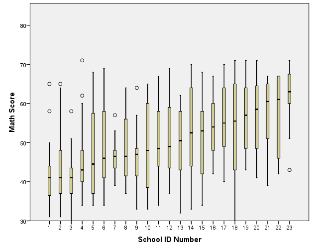
Table 18.2, page 468 Estimated coefficients from three naive linear regression models ignoring the hierarchical structure of the school data. Note that for Model 3, we believe there is a typo where the coefficient for “Three hours” was copied for “Four or more hours”.
*table 18.2, page 468.
glm math with schtype
  /design = schtype
  /print = parameter.

glm math with schtype ses
  /design = schtype ses
  /print = parameter.

glm math with ses schtype  by homew
  /design = schtype ses homew
  /print = parameter.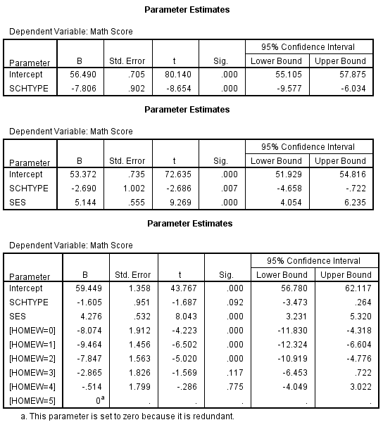
Table 18.3, page 472 Estimated coefficients from three random slope regression models accounting for the hierarchical structure of the school data.
*table 18.3, page 472.
mixed math with schtype
  /fixed=schtype
  /print=solution
  /random=intercept | subject(school).

mixed math with schtype ses
  /fixed=schtype ses
  /print=solution
  /random=intercept | subject(school).

* technically homew 0 should be reference not last.
* the intercept (51) is the first value listed in the estimates table; the parameter estimates for the other
levels of homew are listed in the pairwise comparisons table.
mixed math with schtype ses by homew
  /fixed=schtype ses homew
  /print=solution
  /emmeans = tables(homew) with(schtype = 0) with(ses = 0) compare(homew) refact(first)
  /random=intercept | subject(school).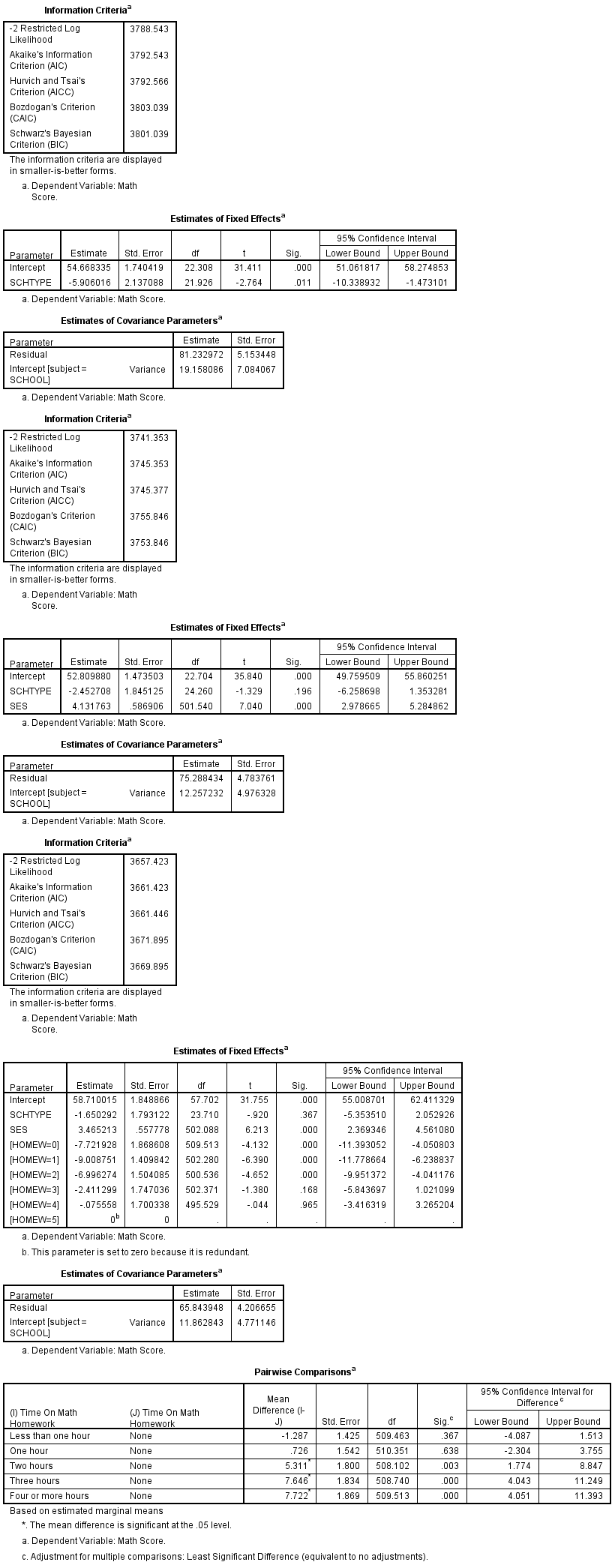
Figure 18.3 is not reproduced.
Table 18.4, page 480
*table 18.4 page 480.
oms select tables
 /destination format = sav numbered = "Table_Number" outfile = "D:pma5Afifi5_mixed.sav"
 /if commands = ['mixed'] subtypes = [' Information Criteria'].

* omit output from all models.
mixed math with sex by race
/fixed=sex race
/random=intercept | subject(school).
mixed math with sex by homew
/fixed=sex homew
/random=intercept | subject(school).
mixed math with sex by ses
/fixed=sex ses
/random=intercept | subject(school).
mixed math with sex by pared
/fixed=sex pared
/random=intercept | subject(school).
mixed math by race homew
/fixed=race homew
/random=intercept | subject(school).
mixed math by race ses
/fixed=race ses
/random=intercept | subject(school).
mixed math by race pared
/fixed=race pared
/random=intercept | subject(school).
mixed math by homew ses
/fixed=homew ses
/random=intercept | subject(school).
mixed math by homew pared
/fixed=homew pared
/random=intercept | subject(school).
mixed math by pared ses
/fixed=pared ses
/random=intercept | subject(school).
omsend.

get file "D:pma5Afifi5_mixed.sav".
delete variables command_ subtype_ label_ .
rename variables table_number = model.
rename variables var1 = ic.
rename variables var2 = value.
select if ic = "Akaike's Information Criterion (AIC)" or ic = "Schwarz's Bayesian Criterion (BIC)".
if missing(value) value = var3.
if missing(value) value = var4.
exe.
delete variables var3 var4.

compute index1 = 1.
if model = lag(model) index1 = lag(index1) + 1.
casestovars
/id = model
/index = index1.
rename variables value.1.00 = AIC.
rename variables value.2.00 = BIC.
exe.
delete variables ic.1.00 ic.2.00.
list.

   model      AIC      BIC

       1 3775.793 3784.282
       2 3704.334 3712.811
       3 2102.648 2109.845
       4 3717.432 3725.908
       5 3685.630 3694.103
       6 2086.811 2094.000
       7 3701.117 3709.590
       8 2048.280 2055.447
       9 3636.012 3644.472
      10 2077.565 2084.732


Number of cases read:  10    Number of cases listed:  10
Figure 18.4, page 483 Weight over time for 14 Mice.
DATASET ACTIVATE Mice.
*figure 18.4, page 483.
GGRAPH
  /GRAPHDATASET NAME="Mice" VARIABLES= day weight id
  /GRAPHSPEC SOURCE=INLINE .
BEGIN GPL
SOURCE: s=userSource( id( "Mice" ) )
DATA: Weight=col( source(s), name( "weight" ) )
DATA: Day=col( source(s), name( "day" ) )
DATA: id=col( source(s), name( "id" ), unit.category() )
GUIDE: text.title( label( "Figure 18.4" ) )
GUIDE: axis( dim( 1 ), label( "Time (Days)" ) )
GUIDE: axis( dim( 2 ), label( "Weight (gr)" ) )
GUIDE: legend( aesthetic( aesthetic.shape.interior ), null() )
ELEMENT: point( position( summary.mode( Day * Weight )  ), shape.interior( id ))
ELEMENT: line( position( summary.mode( Day * Weight )  ), shape.interior( id ))
END GPL.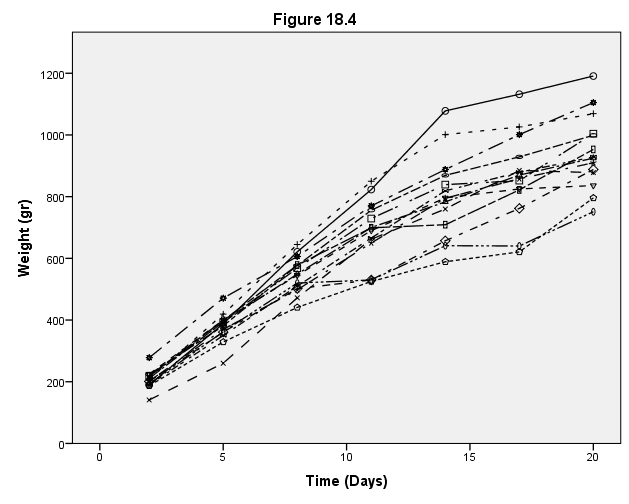
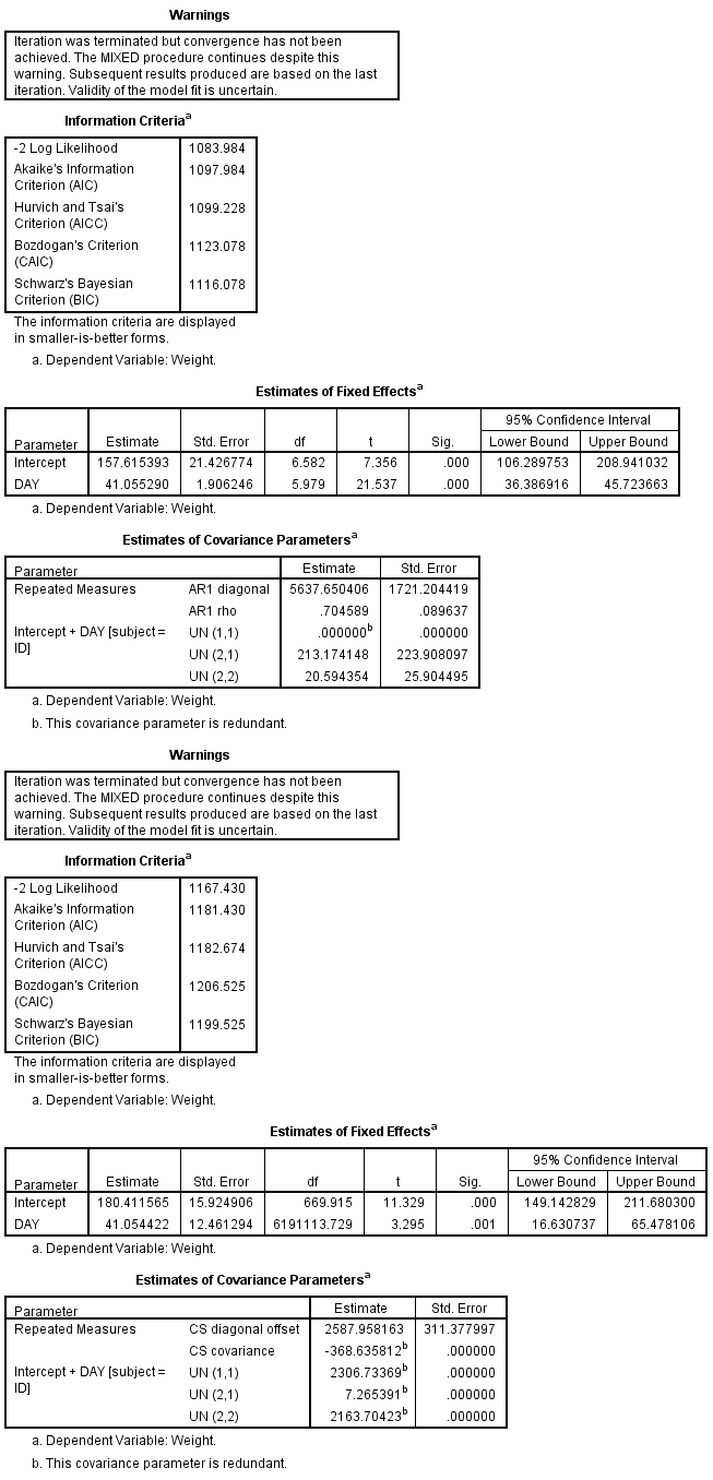
Table 18.5, page 485 Estimates for random intercept and random slope models with different correlation structures. Note that these are complex random effects models to be fitting on only 14 mice. The parameter estimates vary between packages, with some reporting Errors or warnings in the optimization. Note the warnings in SPSS that convergence was not achieved.
*table 18.5, page 485.
* convergence problems with these kind of tricky models given 14 mice.
mixed weight with day
  /criteria mxiter(1000)
  /fixed=day
  /method=ml
  /print=solution
  /random= intercept day | subject(id) covtype(un)
  /repeated= day | subject(id) covtype(ar1).

mixed weight with day
  /fixed=day
  /method=ml
  /print=solution
  /random= intercept day | subject(id) covtype(un)
  /repeated= day | subject(id) covtype(cs).