Page 68 Table 3.1 Regression of postshortage (1981) water use on income and preshortage (1980) water use.
GET FILE 'd:appsrwgdataconcord1.sav'.

REGRESSION
  /DEPENDENT water81
  /METHOD=ENTER income water80.
| Model | Variables Entered | Variables Removed | Method |
|---|---|---|---|
| 1 | Summer 1980 Water Use, Income in Thousands(a) | . | Enter |
| a All requested variables entered. | |||
| b Dependent Variable: Summer 1981 Water Use | |||
| Model | R | R Square | Adjusted R Square | Std. Error of the Estimate |
|---|---|---|---|---|
| 1 | .783(a) | .614 | .612 | 925.428 |
| a Predictors: (Constant), Summer 1980 Water Use, Income in Thousands | ||||
| Model | Sum of Squares | df | Mean Square | F | Sig. | |
|---|---|---|---|---|---|---|
| 1 | Regression | 671025350.237 | 2 | 335512675.119 | 391.763 | .000(a) |
| Residual | 422213359.440 | 493 | 856416.551 | |
|
|
| Total | 1093238709.677 | 495 | |
|
|
|
| a Predictors: (Constant), Summer 1980 Water Use, Income in Thousands | ||||||
| b Dependent Variable: Summer 1981 Water Use | ||||||
| |
Unstandardized Coefficients | Standardized Coefficients | t | Sig. | ||
|---|---|---|---|---|---|---|
| Model | B | Std. Error | Beta | |||
| 1 | (Constant) | 203.822 | 94.361 | |
2.160 | .031 |
| Income in Thousands | 20.545 | 3.383 | .181 | 6.072 | .000 | |
| Summer 1980 Water Use | .593 | .025 | .704 | 23.679 | .000 | |
| a Dependent Variable: Summer 1981 Water Use | ||||||
Page 70 Figure 3.1 Partial regression leverage plot: postshortage water use (Y) versus income (1), adjusting for preshortage water use (2).
REGRESSION
  /DEPENDENT water81
  /METHOD=ENTER water80
 /SAVE RESID.
| Model | Variables Entered | Variables Removed | Method |
|---|---|---|---|
| 1 | Summer 1980 Water Use(a) | . | Enter |
| a All requested variables entered. | |||
| b Dependent Variable: Summer 1981 Water Use | |||
| Model | R | R Square | Adjusted R Square | Std. Error of the Estimate |
|---|---|---|---|---|
| 1 | .765(a) | .585 | .584 | 958.440 |
| a Predictors: (Constant), Summer 1980 Water Use | ||||
| b Dependent Variable: Summer 1981 Water Use | ||||
| Model | Sum of Squares | df | Mean Square | F | Sig. | |
|---|---|---|---|---|---|---|
| 1 | Regression | 639446986.677 | 1 | 639446986.677 | 696.105 | .000(a) |
| Residual | 453791723.000 | 494 | 918606.727 | |
|
|
| Total | 1093238709.677 | 495 | |
|
|
|
| a Predictors: (Constant), Summer 1980 Water Use | ||||||
| b Dependent Variable: Summer 1981 Water Use | ||||||
| |
Unstandardized Coefficients | Standardized Coefficients | t | Sig. | ||
|---|---|---|---|---|---|---|
| Model | B | Std. Error | Beta | |||
| 1 | (Constant) | 537.871 | 79.401 | |
6.774 | .000 |
| Summer 1980 Water Use | .644 | .024 | .765 | 26.384 | .000 | |
| a Dependent Variable: Summer 1981 Water Use | ||||||
| Case Number | Std. Residual | Summer 1981 Water Use |
|---|---|---|
| 25 | 3.283 | 7100 |
| 79 | 3.318 | 8100 |
| 80 | 5.307 | 7300 |
| 85 | 5.548 | 6500 |
| 94 | -5.135 | 3800 |
| 101 | 3.123 | 5400 |
| 118 | 4.992 | 7900 |
| 124 | 4.195 | 10100 |
| 125 | 4.802 | 9200 |
| 325 | 3.316 | 6100 |
| 362 | -3.823 | 1900 |
| a Dependent Variable: Summer 1981 Water Use | ||
| |
Minimum | Maximum | Mean | Std. Deviation | N |
|---|---|---|---|---|---|
| Predicted Value | 666.75 | 8721.65 | 2298.39 | 1136.579 | 496 |
| Residual | -4921.65 | 5317.74 | .00 | 957.471 | 496 |
| Std. Predicted Value | -1.436 | 5.651 | .000 | 1.000 | 496 |
| Std. Residual | -5.135 | 5.548 | .000 | .999 | 496 |
| a Dependent Variable: Summer 1981 Water Use | |||||
REGRESSION
  /DEPENDENT income
  /METHOD=ENTER water80
  /SAVE RESID.
| Model | Variables Entered | Variables Removed | Method |
|---|---|---|---|
| 1 | Summer 1980 Water Use(a) | . | Enter |
| a All requested variables entered. | |||
| b Dependent Variable: Income in Thousands | |||
| Model | R | R Square | Adjusted R Square | Std. Error of the Estimate |
|---|---|---|---|---|
| 1 | .337(a) | .114 | .112 | 12.306 |
| a Predictors: (Constant), Summer 1980 Water Use | ||||
| b Dependent Variable: Income in Thousands | ||||
| Model | Sum of Squares | df | Mean Square | F | Sig. | |
|---|---|---|---|---|---|---|
| 1 | Regression | 9588.317 | 1 | 9588.317 | 63.313 | .000(a) |
| Residual | 74812.772 | 494 | 151.443 | |
|
|
| Total | 84401.089 | 495 | |
|
|
|
| a Predictors: (Constant), Summer 1980 Water Use | ||||||
| b Dependent Variable: Income in Thousands | ||||||
| |
Unstandardized Coefficients | Standardized Coefficients | t | Sig. | ||
|---|---|---|---|---|---|---|
| Model | B | Std. Error | Beta | |||
| 1 | (Constant) | 16.259 | 1.019 | |
15.948 | .000 |
| Summer 1980 Water Use | 2.495E-03 | .000 | .337 | 7.957 | .000 | |
| a Dependent Variable: Income in Thousands | ||||||
| Case Number | Std. Residual | Income in Thousands |
|---|---|---|
| 65 | 3.921 | 72 |
| 118 | 5.181 | 90 |
| 125 | 5.527 | 100 |
| 281 | 3.170 | 68 |
| a Dependent Variable: Income in Thousands | ||
| |
Minimum | Maximum | Mean | Std. Deviation | N |
|---|---|---|---|---|---|
| Predicted Value | 16.76 | 47.95 | 23.08 | 4.401 | 496 |
| Residual | -25.72 | 68.02 | .00 | 12.294 | 496 |
| Std. Predicted Value | -1.436 | 5.651 | .000 | 1.000 | 496 |
| Std. Residual | -2.090 | 5.527 | .000 | .999 | 496 |
| a Dependent Variable: Income in Thousands | |||||
formats res_1 res_2 (f4.0) .
GGRAPH
  /GRAPHDATASET NAME="GraphDataset" VARIABLES= res_1 res_2
  /GRAPHSPEC SOURCE=INLINE .
BEGIN GPL
SOURCE: s=userSource( id( "GraphDataset" ) )
DATA: res_1=col( source(s), name( "res_1" ) )
DATA: res_2=col( source(s), name( "res_2" ) )
COORD: rect( dim( 1, 2 ) )
GUIDE: axis( dim( 1 ), label( "res_2" ) )
GUIDE: axis( dim( 2 ), label( "res_1" ) )
SCALE: linear( dim( 1 ), min(-20), max(60))
SCALE: linear( dim( 2 ), min(-4000), max(4000) )
ELEMENT: point( position(res_2 * res_1 ) )
ELEMENT: line(position( smooth.linear(res_2 * res_1 ) ) )
END GPL.
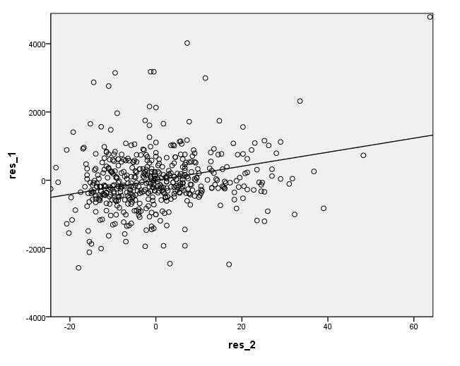
Page 71 Figure 3.2 Partial regression leverage plot: postshortage water use (Y) versus preshortage water use (2), adjusting for income (1).
REGRESSION
  /DEPENDENT water81
  /METHOD=ENTER income
  /SAVE RESID.
| Model | Variables Entered | Variables Removed | Method |
|---|---|---|---|
| 1 | Income in Thousands(a) | . | Enter |
| a All requested variables entered. | |||
| b Dependent Variable: Summer 1981 Water Use | |||
| Model | R | R Square | Adjusted R Square | Std. Error of the Estimate |
|---|---|---|---|---|
| 1 | .418(a) | .175 | .173 | 1351.576 |
| a Predictors: (Constant), Income in Thousands | ||||
| b Dependent Variable: Summer 1981 Water Use | ||||
| Model | Sum of Squares | df | Mean Square | F | Sig. | |
|---|---|---|---|---|---|---|
| 1 | Regression | 190820566.279 | 1 | 190820566.279 | 104.459 | .000(a) |
| Residual | 902418143.398 | 494 | 1826757.375 | |
|
|
| Total | 1093238709.677 | 495 | |
|
|
|
| a Predictors: (Constant), Income in Thousands | ||||||
| b Dependent Variable: Summer 1981 Water Use | ||||||
| |
Unstandardized Coefficients | Standardized Coefficients | t | Sig. | ||
|---|---|---|---|---|---|---|
| Model | B | Std. Error | Beta | |||
| 1 | (Constant) | 1201.124 | 123.325 | |
9.740 | .000 |
| Income in Thousands | 47.549 | 4.652 | .418 | 10.221 | .000 | |
| a Dependent Variable: Summer 1981 Water Use | ||||||
| Case Number | Std. Residual | Summer 1981 Water Use |
|---|---|---|
| 25 | 3.661 | 7100 |
| 62 | 5.187 | 9400 |
| 68 | 3.429 | 7500 |
| 79 | 3.979 | 8100 |
| 108 | 3.661 | 7100 |
| 124 | 5.001 | 10100 |
| 194 | 3.277 | 7200 |
| 446 | 3.161 | 6900 |
| 451 | 4.225 | 8100 |
| a Dependent Variable: Summer 1981 Water Use | ||
| |
Minimum | Maximum | Mean | Std. Deviation | N |
|---|---|---|---|---|---|
| Predicted Value | 1296.22 | 5955.99 | 2298.39 | 620.883 | 496 |
| Residual | -2765.33 | 7010.16 | .00 | 1350.210 | 496 |
| Std. Predicted Value | -1.614 | 5.891 | .000 | 1.000 | 496 |
| Std. Residual | -2.046 | 5.187 | .000 | .999 | 496 |
| a Dependent Variable: Summer 1981 Water Use | |||||
REGRESSION
  /DEPENDENT water80
  /METHOD=ENTER income
  /SAVE RESID.
| Model | Variables Entered | Variables Removed | Method |
|---|---|---|---|
| 1 | Income in Thousands(a) | . | Enter |
| a All requested variables entered. | |||
| b Dependent Variable: Summer 1980 Water Use | |||
| Model | R | R Square | Adjusted R Square | Std. Error of the Estimate |
|---|---|---|---|---|
| 1 | .337(a) | .114 | .112 | 1662.273 |
| a Predictors: (Constant), Income in Thousands | ||||
| b Dependent Variable: Summer 1980 Water Use | ||||
| Model | Sum of Squares | df | Mean Square | F | Sig. | |
|---|---|---|---|---|---|---|
| 1 | Regression | 174943659.340 | 1 | 174943659.340 | 63.313 | .000(a) |
| Residual | 1364996643.080 | 494 | 2763151.099 | |
|
|
| Total | 1539940302.419 | 495 | |
|
|
|
| a Predictors: (Constant), Income in Thousands | ||||||
| b Dependent Variable: Summer 1980 Water Use | ||||||
| |
Unstandardized Coefficients | Standardized Coefficients | t | Sig. | ||
|---|---|---|---|---|---|---|
| Model | B | Std. Error | Beta | |||
| 1 | (Constant) | 1681.433 | 151.674 | |
11.086 | .000 |
| Income in Thousands | 45.528 | 5.722 | .337 | 7.957 | .000 | |
| a Dependent Variable: Summer 1980 Water Use | ||||||
| Case Number | Std. Residual | Summer 1980 Water Use |
|---|---|---|
| 62 | 3.899 | 9300 |
| 94 | 5.396 | 12700 |
| 155 | 3.029 | 7400 |
| 194 | 3.318 | 8700 |
| 362 | 3.407 | 7800 |
| 446 | 3.401 | 8700 |
| 451 | 4.500 | 10300 |
| 477 | 3.073 | 7700 |
| 482 | 3.056 | 7900 |
| a Dependent Variable: Summer 1980 Water Use | ||
| |
Minimum | Maximum | Mean | Std. Deviation | N |
|---|---|---|---|---|---|
| Predicted Value | 1772.49 | 6234.20 | 2732.06 | 594.493 | 496 |
| Residual | -3157.81 | 8969.82 | .00 | 1660.593 | 496 |
| Std. Predicted Value | -1.614 | 5.891 | .000 | 1.000 | 496 |
| Std. Residual | -1.900 | 5.396 | .000 | .999 | 496 |
| a Dependent Variable: Summer 1980 Water Use | |||||
formats res_3 res_4 (f4.0) .
GGRAPH
  /GRAPHDATASET NAME="GraphDataset" VARIABLES= res_3 res_4
  /GRAPHSPEC SOURCE=INLINE .
BEGIN GPL
SOURCE: s=userSource( id( "GraphDataset" ) )
DATA: res_3=col( source(s), name( "res_3" ) )
DATA: res_4=col( source(s), name( "res_4" ) )
GUIDE: axis( dim( 1 ), label( "res_4" ) )
GUIDE: axis( dim( 2 ), label( "res_3" ))
SCALE: linear( dim( 1 ), min(-2000), max(8000))
SCALE: linear( dim( 2 ), min(-2000), max(6000) )
ELEMENT: point( position( res_4 * res_3 ) )
ELEMENT: line(position( smooth.linear(res_4 * res_3 ) ) )
END GPL.
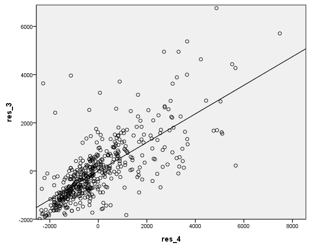
Page 74 Table 3.2 Regression of postshortage water use on income, preshortage water use, education, retirement, number of people in resident, and increase in people in resident.
REGRESSION
  /DEPENDENT water81
  /METHOD=ENTER income water80 educat retire peop81 cpeop.
| Model | Variables Entered | Variables Removed | Method |
|---|---|---|---|
| 1 | Increase in # of People, Education in Years, Summer 1980 Water Use, head of house retired?, Income in Thousands, # of People Resident, 1981(a) | . | Enter |
| a All requested variables entered. | |||
| b Dependent Variable: Summer 1981 Water Use | |||
| Model | R | R Square | Adjusted R Square | Std. Error of the Estimate |
|---|---|---|---|---|
| 1 | .823(a) | .677 | .673 | 849.349 |
| a Predictors: (Constant), Increase in # of People, Education in Years, Summer 1980 Water Use, head of house retired?, Income in Thousands, # of People Resident, 1981 | ||||
| Model | Sum of Squares | df | Mean Square | F | Sig. | |
|---|---|---|---|---|---|---|
| 1 | Regression | 740477522.059 | 6 | 123412920.343 | 171.076 | .000(a) |
| Residual | 352761187.618 | 489 | 721393.022 | |
|
|
| Total | 1093238709.677 | 495 | |
|
|
|
| a Predictors: (Constant), Increase in # of People, Education in Years, Summer 1980 Water Use, head of house retired?, Income in Thousands, # of People Resident, 1981 | ||||||
| b Dependent Variable: Summer 1981 Water Use | ||||||
| |
Unstandardized Coefficients | Standardized Coefficients | t | Sig. | ||
|---|---|---|---|---|---|---|
| Model | B | Std. Error | Beta | |||
| 1 | (Constant) | 242.220 | 206.864 | |
1.171 | .242 |
| Income in Thousands | 20.967 | 3.464 | .184 | 6.053 | .000 | |
| Summer 1980 Water Use | .492 | .026 | .584 | 18.671 | .000 | |
| Education in Years | -41.866 | 13.220 | -.087 | -3.167 | .002 | |
| head of house retired? | 189.184 | 95.021 | .058 | 1.991 | .047 | |
| # of People Resident, 1981 | 248.197 | 28.725 | .277 | 8.641 | .000 | |
| Increase in # of People | 96.454 | 80.519 | .031 | 1.198 | .232 | |
| a Dependent Variable: Summer 1981 Water Use | ||||||
Page 80 Table 3.3 Regression of postshortage water use omitting income and education .
REGRESSION
  /DEPENDENT water81
  /METHOD=ENTER water80 retire peop81 cpeop.
| Model | Variables Entered | Variables Removed | Method |
|---|---|---|---|
| 1 | Increase in # of People, Summer 1980 Water Use, head of house retired?, # of People Resident, 1981(a) | . | Enter |
| a All requested variables entered. | |||
| b Dependent Variable: Summer 1981 Water Use | |||
| Model | R | R Square | Adjusted R Square | Std. Error of the Estimate |
|---|---|---|---|---|
| 1 | .807(a) | .652 | .649 | 880.335 |
| a Predictors: (Constant), Increase in # of People, Summer 1980 Water Use, head of house retired?, # of People Resident, 1981 | ||||
| Model | Sum of Squares | df | Mean Square | F | Sig. | |
|---|---|---|---|---|---|---|
| 1 | Regression | 712718346.262 | 4 | 178179586.565 | 229.912 | .000(a) |
| Residual | 380520363.415 | 491 | 774990.557 | |
|
|
| Total | 1093238709.677 | 495 | |
|
|
|
| a Predictors: (Constant), Increase in # of People, Summer 1980 Water Use, head of house retired?, # of People Resident, 1981 | ||||||
| b Dependent Variable: Summer 1981 Water Use | ||||||
| |
Unstandardized Coefficients | Standardized Coefficients | t | Sig. | ||
|---|---|---|---|---|---|---|
| Model | B | Std. Error | Beta | |||
| 1 | (Constant) | 48.649 | 107.055 | |
.454 | .650 |
| Summer 1980 Water Use | .520 | .027 | .617 | 19.412 | .000 | |
| head of house retired? | 67.280 | 94.288 | .021 | .714 | .476 | |
| # of People Resident, 1981 | 265.289 | 29.632 | .296 | 8.953 | .000 | |
| Increase in # of People | 134.463 | 83.196 | .044 | 1.616 | .107 | |
| a Dependent Variable: Summer 1981 Water Use | ||||||
Page 87 Figure 3.3 Regression of log chloride concentration on a dummy variable for well type.
GET FILE 'd:appsrwgdatawells.sav'.

COMPUTE lnchlor = LG10(chlor).
EXECUTE.

REGRESSION
  /DEPENDENT lnchlor
  /METHOD=ENTER deep.
| Model | Variables Entered | Variables Removed | Method |
|---|---|---|---|
| 1 | bedrock or shallow well?(a) | . | Enter |
| a All requested variables entered. | |||
| b Dependent Variable: LNCHLOR | |||
| Model | R | R Square | Adjusted R Square | Std. Error of the Estimate |
|---|---|---|---|---|
| 1 | .205(a) | .042 | .023 | .58910 |
| a Predictors: (Constant), bedrock or shallow well? | ||||
| Model | Sum of Squares | df | Mean Square | F | Sig. | |
|---|---|---|---|---|---|---|
| 1 | Regression | .759 | 1 | .759 | 2.187 | .145(a) |
| Residual | 17.352 | 50 | .347 | |
|
|
| Total | 18.111 | 51 | |
|
|
|
| a Predictors: (Constant), bedrock or shallow well? | ||||||
| b Dependent Variable: LNCHLOR | ||||||
| |
Unstandardized Coefficients | Standardized Coefficients | t | Sig. | ||
|---|---|---|---|---|---|---|
| Model | B | Std. Error | Beta | |||
| 1 | (Constant) | 1.640 | .186 | |
8.801 | .000 |
| bedrock or shallow well? | -.307 | .207 | -.205 | -1.479 | .145 | |
| a Dependent Variable: LNCHLOR | ||||||
formats deep lnchlor (f1.0).
GGRAPH
  /GRAPHDATASET NAME="GraphDataset" VARIABLES= lnchlor deep
  /GRAPHSPEC SOURCE=INLINE.
BEGIN GPL
SOURCE: s=userSource( id( "GraphDataset" ) )
DATA: lnchlor=col( source(s), name( "lnchlor" ) )
DATA: deep=col( source(s), name( "deep" ) )
GUIDE: axis( dim( 1 ), label( "Well Type" ), delta(1) )
GUIDE: axis( dim( 2 ), label( "Natural Log of Cholride Consentration" ) )
SCALE: linear( dim( 1 ), min(0), max(1) )
SCALE: linear( dim( 2 ), min(1), max(6) )
ELEMENT: point( position( deep * lnchlor ) )
ELEMENT: line(position( smooth.linear(deep * lnchlor ) ) )
END GPL.
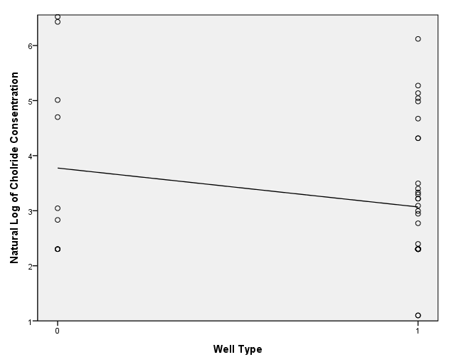
Page 88 Figure 3.4 Regression of log chloride concentration on log distance from road and an intercept dummy variable for well type.
COMPUTE LNROAD=LG10(DROAD).
EXECUTE.

REGRESSION
  /DEPENDENT lnchlor deep
  /METHOD=ENTER lnroad
  /SAVE pred (pred1).
|
Variables Entered/Removedb |
|||
|
Model |
Variables Entered |
Variables Removed |
Method |
|
1 |
deep bedrock or shallow well?, LNROADa |
. |
Enter |
|
a. All requested variables entered. |
|||
|
b. Dependent Variable: lnchlor |
|||
|
Model Summaryb |
||||
|
Model |
R |
R Square |
Adjusted R Square |
Std. Error of the Estimate |
|
1 |
.217a |
.047 |
.008 |
1.36666 |
|
a. Predictors: (Constant), deep bedrock or shallow well?, LNROAD |
||||
|
b. Dependent Variable: lnchlor |
||||
|
ANOVAb |
||||||
|
Model |
Sum of Squares |
df |
Mean Square |
F |
Sig. |
|
|
1 |
Regression |
4.502 |
2 |
2.251 |
1.205 |
.308a |
|
Residual |
91.520 |
49 |
1.868 |
|||
|
Total |
96.022 |
51 |
||||
|
a. Predictors: (Constant), deep bedrock or shallow well?, LNROAD |
||||||
|
b. Dependent Variable: lnchlor |
||||||
|
Coefficientsa |
||||||
|
Model |
Unstandardized Coefficients |
Standardized Coefficients |
t |
Sig. |
||
|
B |
Std. Error |
Beta |
||||
|
1 |
(Constant) |
4.210 |
.961 |
4.381 |
.000 |
|
|
LNROAD |
-.091 |
.180 |
-.071 |
-.506 |
.615 |
|
|
deep bedrock or shallow well? |
-.697 |
.481 |
-.202 |
-1.449 |
.154 |
|
|
a. Dependent Variable: lnchlor |
||||||
|
Residuals Statisticsa |
|||||
|
Minimum |
Maximum |
Mean |
Std. Deviation |
N |
|
|
Predicted Value |
2.7957 |
3.8861 |
3.2050 |
.29711 |
52 |
|
Residual |
-2.05794 |
3.78616 |
.00000 |
1.33960 |
52 |
|
Std. Predicted Value |
-1.378 |
2.292 |
.000 |
1.000 |
52 |
|
Std. Residual |
-1.506 |
2.770 |
.000 |
.980 |
52 |
|
a. Dependent Variable: lnchlor |
|||||
formats lnroad lnchlor pred1 (f1.0).
GGRAPH
  /GRAPHDATASET NAME="graphdataset" VARIABLES=lnroad lnchlor deep pred1
  /GRAPHSPEC SOURCE=INLINE.
BEGIN GPL
SOURCE: s=userSource(id("graphdataset"))
DATA: lnroad=col(source(s), name("lnroad"))
DATA: pred1=col(source(s), name("pred1"))
DATA: deep=col(source(s), name("deep"), unit.category() )
DATA: lnchlor=col(source(s), name("lnchlor"))
GUIDE: axis( dim( 1 ), label( "natural log distance from road" ), delta(2) )
GUIDE: axis( dim( 2 ), label( "natural log of cholride consentration" ), delta(1) )
SCALE: linear( dim( 1 ), min(0), max(8) )
SCALE: linear( dim( 2 ), min(0), max(7) )
ELEMENT: point(position(lnroad*lnchlor))
ELEMENT: line(position( smooth.linear(lnroad * pred1 ) ), shape(deep) )
END GPL.
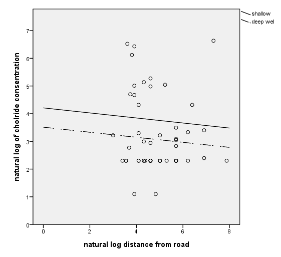
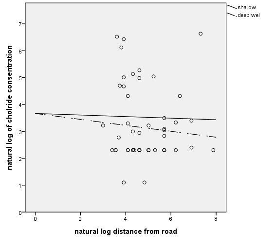
Page 89 Figure 3.5 Regression of log chloride concentration on log distance from road and a slope dummy variable for well type.
Compute deeproad=deep*lnroad.
Execute.

REGRESSION
 /DEPENDENT lnchlor
 /METHOD=ENTER lnroad deeproad
 /SAVE pred (pred2).
|
Variables Entered/Removedb |
|||
|
Model |
Variables Entered |
Variables Removed |
Method |
|
1 |
deeproad, LNROADa |
. |
Enter |
|
a. All requested variables entered. |
|||
|
b. Dependent Variable: lnchlor |
|||
|
Model Summaryb |
||||
|
Model |
R |
R Square |
Adjusted R Square |
Std. Error of the Estimate |
|
1 |
.140a |
.019 |
-.021 |
1.386 |
|
a. Predictors: (Constant), deeproad, LNROAD |
||||
|
b. Dependent Variable: lnchlor |
||||
|
ANOVAb |
||||||
|
Model |
Sum of Squares |
df |
Mean Square |
F |
Sig. |
|
|
1 |
Regression |
1.871 |
2 |
.935 |
.487 |
.618a |
|
Residual |
94.151 |
49 |
1.921 |
|||
|
Total |
96.022 |
51 |
||||
|
a. Predictors: (Constant), deeproad, LNROAD |
||||||
|
b. Dependent Variable: lnchlor |
||||||
|
Coefficientsa |
||||||
|
Model |
Unstandardized Coefficients |
Standardized Coefficients |
t |
Sig. |
||
|
B |
Std. Error |
Beta |
||||
|
1 |
(Constant) |
3.666 |
.905 |
4.050 |
.000 |
|
|
LNROAD |
-.029 |
.202 |
-.022 |
-.144 |
.886 |
|
|
deeproad |
-.081 |
.099 |
-.128 |
-.819 |
.417 |
|
|
a. Dependent Variable: lnchlor |
||||||
|
Residuals Statisticsa |
|||||
|
Minimum |
Maximum |
Mean |
Std. Deviation |
N |
|
|
Predicted Value |
2.80 |
3.56 |
3.21 |
.192 |
52 |
|
Residual |
-2.135 |
3.775 |
.000 |
1.359 |
52 |
|
Std. Predicted Value |
-2.135 |
1.870 |
.000 |
1.000 |
52 |
|
Std. Residual |
-1.541 |
2.723 |
.000 |
.980 |
52 |
|
a. Dependent Variable: lnchlor |
|||||
formats lnroad lnchlor pred2 (f1.0).
GGRAPH
  /GRAPHDATASET NAME="graphdataset" VARIABLES=lnroad lnchlor deep pred2
  /GRAPHSPEC SOURCE=INLINE.
BEGIN GPL
SOURCE: s=userSource(id("graphdataset"))
DATA: lnroad=col(source(s), name("lnroad"))
DATA: pred2=col(source(s), name("pred2"))
DATA: deep=col(source(s), name("deep"), unit.category() )
DATA: lnchlor=col(source(s), name("lnchlor"))
GUIDE: axis( dim( 1 ), label( "natural log distance from road" ), delta(2) )
GUIDE: axis( dim( 2 ), label( "natural log of cholride consentration" ), delta(1) )
SCALE: linear( dim( 1 ), min(0), max(8) )
SCALE: linear( dim( 2 ), min(0), max(7) )
ELEMENT: point(position(lnroad*lnchlor))
ELEMENT: line(position( smooth.linear(lnroad * pred2 ) ), shape(deep) )
END GPL.
Page 90 Table 3.4 Regression of log chloride concentration on log distance from road, with intercept and slope dummy variables for well type.
REGRESSION
/DEPENDENT lnchlor
/METHOD=ENTER deep lnroad deeproad.
| Model | Variables Entered | Variables Removed | Method |
|---|---|---|---|
| 1 | DEEPROAD, LNROAD, bedrock or shallow well?(a) | . | Enter |
| a All requested variables entered. | |||
| b Dependent Variable: LNCHLOR | |||
| Model | R | R Square | Adjusted R Square | Std. Error of the Estimate |
|---|---|---|---|---|
| 1 | .439(a) | .192 | .142 | .55198 |
| a Predictors: (Constant), DEEPROAD, LNROAD, bedrock or shallow well? | ||||
| Model | Sum of Squares | df | Mean Square | F | Sig. | |
|---|---|---|---|---|---|---|
| 1 | Regression | 3.486 | 3 | 1.162 | 3.814 | .016(a) |
| Residual | 14.625 | 48 | .305 | |
|
|
| Total | 18.111 | 51 | |
|
|
|
| a Predictors: (Constant), DEEPROAD, LNROAD, bedrock or shallow well? | ||||||
| b Dependent Variable: LNCHLOR | ||||||
| |
Unstandardized Coefficients | Standardized Coefficients | t | Sig. | ||
|---|---|---|---|---|---|---|
| Model | B | Std. Error | Beta | |||
| 1 | (Constant) | 3.941 | .816 | |
4.828 | .000 |
| bedrock or shallow well? | -2.917 | .910 | -1.948 | -3.207 | .002 | |
| LNROAD | -1.109 | .384 | -.862 | -2.886 | .006 | |
| DEEPROAD | 1.256 | .427 | 1.979 | 2.942 | .005 | |
| a Dependent Variable: LNCHLOR | ||||||
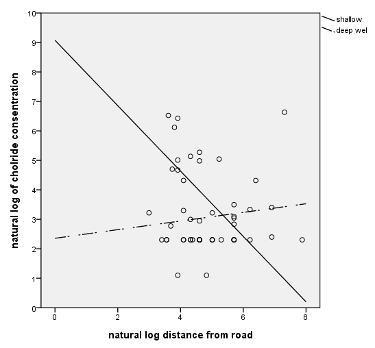
Page 91 Figure 3.6 Regression of log chloride concentration on log distance from road, with slope and intercept dummy variables for well type.
GGRAPH
  /GRAPHDATASET NAME="graphdataset" VARIABLES=lnroad lnchlor deep
  /GRAPHSPEC SOURCE=INLINE.
BEGIN GPL
SOURCE: s=userSource(id("graphdataset"))
DATA: lnroad=col(source(s), name("lnroad"))
DATA: deep=col(source(s), name("deep"), unit.category() )
DATA: lnchlor=col(source(s), name("lnchlor"))
GUIDE: axis( dim( 1 ), label( "natural log distance from road" ), delta(2) )
GUIDE: axis( dim( 2 ), label( "natural log of cholride consentration" ), delta(1) )
SCALE: linear( dim( 1 ), min(0), max(8) )
SCALE: linear( dim( 2 ), min(0), max(9) )
ELEMENT: point(position(lnroad*lnchlor))
ELEMENT: line(position( smooth.linear(lnroad * lnchlor ) ), shape(deep) )
END GPL.
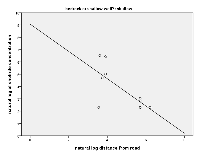
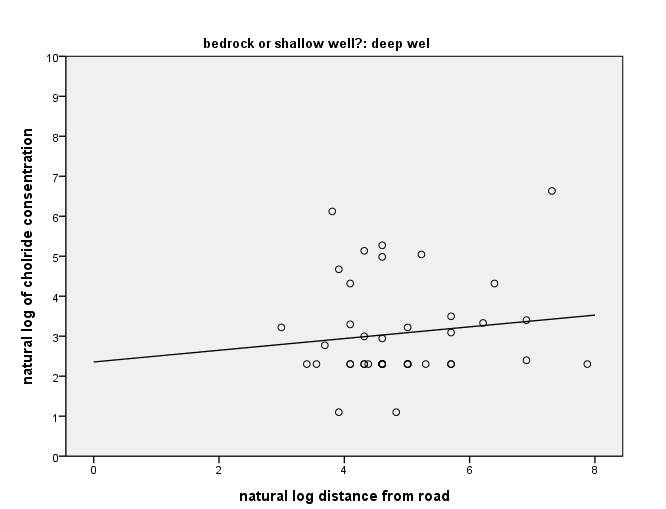
Page 91 Figure 3.7 Separate regression for shallow (left) and deep (right) wells; same line as in Figure 3.6.
sort cases by deep.
split file by deep.
GGRAPH
  /GRAPHDATASET NAME="graphdataset" VARIABLES=lnroad lnchlor
  /GRAPHSPEC SOURCE=INLINE.
BEGIN GPL
SOURCE: s=userSource(id("graphdataset"))
DATA: lnroad=col(source(s), name("lnroad"))
DATA: lnchlor=col(source(s), name("lnchlor"))
GUIDE: axis( dim( 1 ), label( "natural log distance from road" ), delta(2) )
GUIDE: axis( dim( 2 ), label( "natural log of cholride consentration" ), delta(1) )
SCALE: linear( dim( 1 ), min(0), max(8) )
SCALE: linear( dim( 2 ), min(0), max(9) )
ELEMENT: point(position(lnroad*lnchlor))
ELEMENT: line(position( smooth.linear(lnroad * lnchlor ) ) )
END GPL.
split file off.
Page 93 Table 3.5 Cancer, bedrock and radon in 26 counties.
GET FILE 'd:appsrwgdataradon.sav'.

USE ALL.
SELECT IF(number > 0).
EXECUTE.

if reading=1 area=1.
if fringe=1 area=2.
if control=1 area=3.

recode radon (0 thru 1.5=1) into mnradon.
recode radon (1.6 thru 2.45=2) into mnradon.
recode radon (2.5 thru 10.0=3) into mnradon.

compute lowradon=0.
if mnradon=1 lowradon=1.
compute midradon=0.
if mnradon=2 midradon=1.
execute.

list county cancer locale reading fringe mnradon lowradon midradon.
COUNTY         CANCER   LOCALE  READING   FRINGE  MNRADON LOWRADON MIDRADON

Orange           6.00        1        1        0     1.00     1.00      .00
Putnam          10.50        1        1        0     2.00      .00     1.00
Sussex           6.70        1        1        0     2.00      .00     1.00
Warren           6.00        1        1        0     3.00      .00      .00
Morris           6.10        1        1        0     1.00     1.00      .00
Hunterdon        6.70        1        1        0     3.00      .00      .00
Berks            5.20        2        0        1     3.00      .00      .00
Lehigh           5.60        2        0        1     3.00      .00      .00
Northampton      5.80        2        0        1     3.00      .00      .00
Pike             4.50        2        0        1     1.00     1.00      .00
Dutchess         5.50        2        0        1     2.00      .00     1.00
Sullivan         5.40        2        0        1     1.00     1.00      .00
Ulster           6.30        2        0        1     1.00     1.00      .00
Columbia         6.30        3        0        0     2.00      .00     1.00
Delaware         4.30        3        0        0     2.00      .00     1.00
Greene           4.00        3        0        0     2.00      .00     1.00
Otsego           5.90        3        0        0     2.00      .00     1.00
Tioga            4.70        3        0        0     2.00      .00     1.00
Carbon           4.80        3        0        0     2.00      .00     1.00
Lebanon          5.80        3        0        0     3.00      .00      .00
Lackawanna       5.40        3        0        0     1.00     1.00      .00
Luzerne          5.20        3        0        0     1.00     1.00      .00
Schuylkill       3.60        3        0        0     3.00      .00      .00
Susquehanna      4.30        3        0        0     1.00     1.00      .00
Wayne            3.50        3        0        0     1.00     1.00      .00
Wyoming          6.90        3        0        0     2.00      .00     1.00

Number of cases read:  26    Number of cases listed:  26
Page 94 Table 3.6 Relation between cancer rate and bedrock area.
REGRESSION
  /VAR=cancer reading fringe
  /DEPENDENT cancer
  /METHOD=TEST(reading fringe).
| Model | Variables Entered | Variables Removed | Method |
|---|---|---|---|
| 1 | Fringe area dummy, Reading Prong dummy | . | Test |
| a Dependent Variable: Wt.Female Lung Cancer (x10^-5/y | |||
| Model | R | R Square | Adjusted R Square | Std. Error of the Estimate |
|---|---|---|---|---|
| 1 | .598(a) | .358 | .302 | 1.14848 |
| a Predictors: (Constant), Fringe area dummy, Reading Prong dummy | ||||
| Model | Sum of Squares | df | Mean Square | F | Sig. | R Square Change | ||
|---|---|---|---|---|---|---|---|---|
| 1 | Subset Tests | Reading Prong dummy, Fringe area dummy | 16.909 | 2 | 8.454 | 6.410 | .006(a) | .358 |
| Regression | 16.909 | 2 | 8.454 | 6.410 | .006(b) | |
||
| Residual | 30.337 | 23 | 1.319 | |
|
|
||
| Total | 47.246 | 25 | |
|
|
|
||
| a Tested against the full model. | ||||||||
| b Predictors in the Full Model: (Constant), Fringe area dummy, Reading Prong dummy. | ||||||||
| c Dependent Variable: Wt.Female Lung Cancer (x10^-5/y | ||||||||
| |
Unstandardized Coefficients | Standardized Coefficients | t | Sig. | ||
|---|---|---|---|---|---|---|
| Model | B | Std. Error | Beta | |||
| 1 | (Constant) | 4.977 | .319 | |
15.625 | .000 |
| Reading Prong dummy | 2.023 | .567 | .632 | 3.569 | .002 | |
| Fringe area dummy | .495 | .538 | .163 | .918 | .368 | |
| a Dependent Variable: Wt.Female Lung Cancer (x10^-5/y | ||||||
ONEWAY
  cancer BY area.
| |
Sum of Squares | df | Mean Square | F | Sig. |
|---|---|---|---|---|---|
| Between Groups | 16.909 | 2 | 8.454 | 6.410 | .006 |
| Within Groups | 30.337 | 23 | 1.319 | |
|
| Total | 47.246 | 25 | |
|
|
Page 96 Table 3.7 Relation among cancer rate, bedrock area, and radon.
REGRESSION
  /VAR=cancer reading fringe lowradon midradon
  /DEPENDENT cancer
  /METHOD=TEST(reading fringe) (lowradon midradon).
| Model | Variables Entered | Variables Removed | Method |
|---|---|---|---|
| 1 | MIDRADON, Reading Prong dummy, Fringe area dummy, LOWRADON | . | Test |
| a Dependent Variable: Wt.Female Lung Cancer (x10^-5/y | |||
| Model | R | R Square | Adjusted R Square | Std. Error of the Estimate |
|---|---|---|---|---|
| 1 | .684(a) | .468 | .367 | 1.09376 |
| a Predictors: (Constant), MIDRADON, Reading Prong dummy, Fringe area dummy, LOWRADON | ||||
| Model | Sum of Squares | df | Mean Square | F | Sig. | R Square Change | ||
|---|---|---|---|---|---|---|---|---|
| 1 | Subset Tests | Reading Prong dummy, Fringe area dummy | 19.285 | 2 | 9.642 | 8.060 | .003(a) | .408 |
| LOWRADON, MIDRADON | 5.215 | 2 | 2.607 | 2.180 | .138(a) | .110 | ||
| Regression | 22.124 | 4 | 5.531 | 4.623 | .008(b) | |
||
| Residual | 25.123 | 21 | 1.196 | |
|
|
||
| Total | 47.246 | 25 | |
|
|
|
||
| a Tested against the full model. | ||||||||
| b Predictors in the Full Model: (Constant), MIDRADON, Reading Prong dummy, Fringe area dummy, LOWRADON. | ||||||||
| c Dependent Variable: Wt.Female Lung Cancer (x10^-5/y | ||||||||
| |
Unstandardized Coefficients | Standardized Coefficients | t | Sig. | ||
|---|---|---|---|---|---|---|
| Model | B | Std. Error | Beta | |||
| 1 | (Constant) | 4.525 | .528 | |
8.569 | .000 |
| Reading Prong dummy | 2.212 | .551 | .691 | 4.014 | .001 | |
| Fringe area dummy | .867 | .549 | .285 | 1.579 | .129 | |
| LOWRADON | -.117 | .556 | -.041 | -.210 | .836 | |
| MIDRADON | .906 | .576 | .327 | 1.573 | .131 | |
| a Dependent Variable: Wt.Female Lung Cancer (x10^-5/y | ||||||
UNIANOVA
  cancer  BY area mnradon
  /DESIGN = area mnradon.
| |
N | |
|---|---|---|
| AREA | 1.00 | 6 |
| 2.00 | 7 | |
| 3.00 | 13 | |
| MNRADON | 1.00 | 9 |
| 2.00 | 10 | |
| 3.00 | 7 | |
| Source | Type III Sum of Squares | df | Mean Square | F | Sig. |
|---|---|---|---|---|---|
| Corrected Model | 22.124(a) | 4 | 5.531 | 4.623 | .008 |
| Intercept | 784.039 | 1 | 784.039 | 655.380 | .000 |
| AREA | 19.285 | 2 | 9.642 | 8.060 | .003 |
| MNRADON | 5.215 | 2 | 2.607 | 2.180 | .138 |
| Error | 25.123 | 21 | 1.196 | |
|
| Total | 855.900 | 26 | |
|
|
| Corrected Total | 47.246 | 25 | |
|
|
| a R Squared = .468 (Adjusted R Squared = .367) | |||||
Page 98 Table 3.8 Relation among cancer rate, bedrock area, and radon, with interaction.
compute x1x3=reading*lowradon.
compute x1x4=reading*midradon.
compute x2x3=fringe*lowradon.
compute x2x4=fringe*midradon.
execute.

REGRESSION
  /VAR cancer reading fringe lowradon midradon x1x3 x1x4 x2x3 x2x4
  /DEPENDENT cancer
  /METHOD=TEST(reading fringe lowradon midradon) (x1x3 x1x4 x2x3 x2x4).
| Model | Variables Entered | Variables Removed | Method |
|---|---|---|---|
| 1 | X2X4, X1X4, X1X3, X2X3, MIDRADON, LOWRADON, Fringe area dummy, Reading Prong dummy | . | Test |
| a Dependent Variable: Wt.Female Lung Cancer (x10^-5/y | |||
| Model | R | R Square | Adjusted R Square | Std. Error of the Estimate |
|---|---|---|---|---|
| 1 | .742(a) | .551 | .340 | 1.11701 |
| a Predictors: (Constant), X2X4, X1X4, X1X3, X2X3, MIDRADON, LOWRADON, Fringe area dummy, Reading Prong dummy | ||||
| Model | Sum of Squares | df | Mean Square | F | Sig. | R Square Change | ||
|---|---|---|---|---|---|---|---|---|
| 1 | Subset Tests | Reading Prong dummy, Fringe area dummy, LOWRADON, MIDRADON | 4.945 | 4 | 1.236 | .991 | .439(a) | .105 |
| X1X3, X1X4, X2X3, X2X4 | 3.912 | 4 | .978 | .784 | .551(a) | .083 | ||
| Regression | 26.035 | 8 | 3.254 | 2.608 | .046(b) | |
||
| Residual | 21.211 | 17 | 1.248 | |
|
|
||
| Total | 47.246 | 25 | |
|
|
|
||
| a Tested against the full model. | ||||||||
| b Predictors in the Full Model: (Constant), X2X4, X1X4, X1X3, X2X3, MIDRADON, LOWRADON, Fringe area dummy, Reading Prong dummy. | ||||||||
| c Dependent Variable: Wt.Female Lung Cancer (x10^-5/y | ||||||||
| |
Unstandardized Coefficients | Standardized Coefficients | t | Sig. | ||
|---|---|---|---|---|---|---|
| Model | B | Std. Error | Beta | |||
| 1 | (Constant) | 4.700 | .790 | |
5.951 | .000 |
| Reading Prong dummy | 1.650 | 1.117 | .516 | 1.477 | .158 | |
| Fringe area dummy | .833 | 1.020 | .274 | .817 | .425 | |
| LOWRADON | -.100 | .967 | -.035 | -.103 | .919 | |
| MIDRADON | .571 | .896 | .206 | .638 | .532 | |
| X1X3 | -.200 | 1.478 | -.040 | -.135 | .894 | |
| X1X4 | 1.679 | 1.432 | .332 | 1.172 | .257 | |
| X2X3 | -3.333E-02 | 1.330 | -.008 | -.025 | .980 | |
| X2X4 | -.605 | 1.570 | -.086 | -.385 | .705 | |
| a Dependent Variable: Wt.Female Lung Cancer (x10^-5/y | ||||||
UNIANOVA  cancer  BY area mnradon
  /DESIGN = area mnradon area*mnradon.
| |
N | |
|---|---|---|
| AREA | 1.00 | 6 |
| 2.00 | 7 | |
| 3.00 | 13 | |
| MNRADON | 1.00 | 9 |
| 2.00 | 10 | |
| 3.00 | 7 | |
| Source | Type III Sum of Squares | df | Mean Square | F | Sig. |
|---|---|---|---|---|---|
| Corrected Model | 26.035(a) | 8 | 3.254 | 2.608 | .046 |
| Intercept | 666.210 | 1 | 666.210 | 533.949 | .000 |
| AREA | 17.400 | 2 | 8.700 | 6.973 | .006 |
| MNRADON | 4.358 | 2 | 2.179 | 1.746 | .204 |
| AREA * MNRADON | 3.912 | 4 | .978 | .784 | .551 |
| Error | 21.211 | 17 | 1.248 | |
|
| Total | 855.900 | 26 | |
|
|
| Corrected Total | 47.246 | 25 | |
|
|
| a R Squared = .551 (Adjusted R Squared = .340) | |||||
Page 99 Table 3.9 Effect coding of bedrock area from Table 3.5.
if area=1 rev1=1.
if area=2 rev1=0.
if area=3 rev1=-1.
if area=1 fev2=0.
if area=2 fev2=1.
if area=3 fev2=-1.
execute.

list county area reading ereading fringe efringe.
COUNTY          AREA  READING EREADING   FRINGE  EFRINGE

Orange          1.00        1        1        0        0
Putnam          1.00        1        1        0        0
Sussex          1.00        1        1        0        0
Warren          1.00        1        1        0        0
Morris          1.00        1        1        0        0
Hunterdon       1.00        1        1        0        0
Berks           2.00        0        0        1        1
Lehigh          2.00        0        0        1        1
Northampton     2.00        0        0        1        1
Pike            2.00        0        0        1        1
Dutchess        2.00        0        0        1        1
Sullivan        2.00        0        0        1        1
Ulster          2.00        0        0        1        1
Columbia        3.00        0       -1        0       -1
Delaware        3.00        0       -1        0       -1
Greene          3.00        0       -1        0       -1
Otsego          3.00        0       -1        0       -1
Tioga           3.00        0       -1        0       -1
Carbon          3.00        0       -1        0       -1
Lebanon         3.00        0       -1        0       -1
Lackawanna      3.00        0       -1        0       -1
Luzerne         3.00        0       -1        0       -1
Schuylkill      3.00        0       -1        0       -1
Susquehanna     3.00        0       -1        0       -1
Wayne           3.00        0       -1        0       -1
Wyoming         3.00        0       -1        0       -1

Number of cases read:  26    Number of cases listed:  26
Page 100 Table 3.10 Relation among cancer rate, bedrock area, and radon.
compute v3=lowradon.
if mnradon=3 v3=-1.
compute v4=midradon.
if mnradon=3 v4=-1.
compute v1v3=ereading*v3.
compute v1v4=ereading*v4.
compute v2v3=efringe*v3.
compute v2v4=efringe*v4.
execute.

REGRESSION
 /VAR cancer ereading efringe v3 v4 v1v3 v1v4 v2v3 v2v4
 /DEPENDENT cancer
 /METHOD=TEST (ereading efringe v3 v4) (v1v3 v1v4 v2v3 v2v4).
| Model | Variables Entered | Variables Removed | Method |
|---|---|---|---|
| 1 | V2V4, effects-coded fringe, V3, V1V3, V2V3, effects-coded Reading, V4, V1V4 | . | Test |
| a Dependent Variable: Wt.Female Lung Cancer (x10^-5/y | |||
| Model | R | R Square | Adjusted R Square | Std. Error of the Estimate |
|---|---|---|---|---|
| 1 | .742(a) | .551 | .340 | 1.11701 |
| a Predictors: (Constant), V2V4, effects-coded fringe, V3, V1V3, V2V3, effects-coded Reading, V4, V1V4 | ||||
| Model | Sum of Squares | df | Mean Square | F | Sig. | R Square Change | ||
|---|---|---|---|---|---|---|---|---|
| 1 | Subset Tests | effects-coded Reading, effects-coded fringe, V3, V4 | 21.612 | 4 | 5.403 | 4.330 | .013(a) | .457 |
| V1V3, V1V4, V2V3, V2V4 | 3.912 | 4 | .978 | .784 | .551(a) | .083 | ||
| Regression | 26.035 | 8 | 3.254 | 2.608 | .046(b) | |
||
| Residual | 21.211 | 17 | 1.248 | |
|
|
||
| Total | 47.246 | 25 | |
|
|
|
||
| a Tested against the full model. | ||||||||
| b Predictors in the Full Model: (Constant), V2V4, effects-coded fringe, V3, V1V3, V2V3, effects-coded Reading, V4, V1V4. | ||||||||
| c Dependent Variable: Wt.Female Lung Cancer (x10^-5/y | ||||||||
| |
Unstandardized Coefficients | Standardized Coefficients | t | Sig. | ||
|---|---|---|---|---|---|---|
| Model | B | Std. Error | Beta | |||
| 1 | (Constant) | 5.778 | .250 | |
23.107 | .000 |
| effects-coded Reading | 1.222 | .363 | .735 | 3.365 | .004 | |
| effects-coded fringe | -.301 | .374 | -.189 | -.804 | .432 | |
| V3 | -.428 | .336 | -.248 | -1.276 | .219 | |
| V4 | .679 | .372 | .403 | 1.824 | .086 | |
| V1V3 | -.522 | .501 | -.238 | -1.041 | .313 | |
| V1V4 | .921 | .526 | .465 | 1.750 | .098 | |
| V2V3 | .351 | .486 | .176 | .722 | .480 | |
| V2V4 | -.657 | .595 | -.318 | -1.103 | .285 | |
| a Dependent Variable: Wt.Female Lung Cancer (x10^-5/y | ||||||
UNIANOVA  cancer  BY area mnradon
  /DESIGN = area mnradon area*mnradon.
| |
N | |
|---|---|---|
| AREA | 1.00 | 6 |
| 2.00 | 7 | |
| 3.00 | 13 | |
| MNRADON | 1.00 | 9 |
| 2.00 | 10 | |
| 3.00 | 7 | |
| Source | Type III Sum of Squares | df | Mean Square | F | Sig. |
|---|---|---|---|---|---|
| Corrected Model | 26.035(a) | 8 | 3.254 | 2.608 | .046 |
| Intercept | 666.210 | 1 | 666.210 | 533.949 | .000 |
| AREA | 17.400 | 2 | 8.700 | 6.973 | .006 |
| MNRADON | 4.358 | 2 | 2.179 | 1.746 | .204 |
| AREA * MNRADON | 3.912 | 4 | .978 | .784 | .551 |
| Error | 21.211 | 17 | 1.248 | |
|
| Total | 855.900 | 26 | |
|
|
| Corrected Total | 47.246 | 25 | |
|
|
| a R Squared = .551 (Adjusted R Squared = .340) | |||||
