Page 114 Table 4.2 Correlation matrix for 1981 household water use and predictors.
GET FILE 'd:concord1.sav'.

CORRELATIONS
 /VARIABLES=income water80 educat retire peop81 cpeop water81
 /PRINT=TWOTAIL SIG.
Correlations
| |
Income in Thousands | Summer 1980 Water Use | Education in Years | head of house retired? | # of People Resident, 1981 | Increase in # of People | Summer 1981 Water Use | |
|---|---|---|---|---|---|---|---|---|
| Income in Thousands | Pearson Correlation | 1 | .337 | .346 | -.381 | .311 | .091 | .418 |
| Sig. (2-tailed) | . | .000 | .000 | .000 | .000 | .043 | .000 | |
| N | 496 | 496 | 496 | 496 | 496 | 496 | 496 | |
| Summer 1980 Water Use | Pearson Correlation | .337 | 1 | .098 | -.292 | .525 | -.031 | .765 |
| Sig. (2-tailed) | .000 | . | .029 | .000 | .000 | .489 | .000 | |
| N | 496 | 496 | 496 | 496 | 496 | 496 | 496 | |
| Education in Years | Pearson Correlation | .346 | .098 | 1 | -.174 | .059 | .005 | .040 |
| Sig. (2-tailed) | .000 | .029 | . | .000 | .192 | .903 | .370 | |
| N | 496 | 496 | 496 | 496 | 496 | 496 | 496 | |
| head of house retired? | Pearson Correlation | -.381 | -.292 | -.174 | 1 | -.376 | -.059 | -.273 |
| Sig. (2-tailed) | .000 | .000 | .000 | . | .000 | .193 | .000 | |
| N | 496 | 496 | 496 | 496 | 496 | 496 | 496 | |
| # of People Resident, 1981 | Pearson Correlation | .311 | .525 | .059 | -.376 | 1 | .144 | .618 |
| Sig. (2-tailed) | .000 | .000 | .192 | .000 | . | .001 | .000 | |
| N | 496 | 496 | 496 | 496 | 496 | 496 | 496 | |
| Increase in # of People | Pearson Correlation | .091 | -.031 | .005 | -.059 | .144 | 1 | .066 |
| Sig. (2-tailed) | .043 | .489 | .903 | .193 | .001 | . | .142 | |
| N | 496 | 496 | 496 | 496 | 496 | 496 | 496 | |
| Summer 1981 Water Use | Pearson Correlation | .418 | .765 | .040 | -.273 | .618 | .066 | 1 |
| Sig. (2-tailed) | .000 | .000 | .370 | .000 | .000 | .142 | . | |
| N | 496 | 496 | 496 | 496 | 496 | 496 | 496 | |
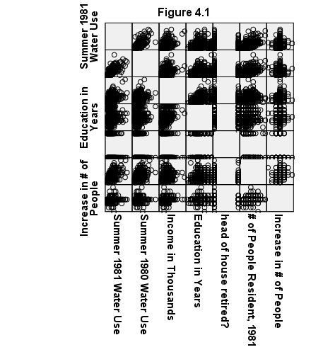
Page 115 Figure 4.1 Scatterplot matrix corresponding to Table 4.2 (household water use and predictors).
GGRAPH
  /GRAPHDATASET NAME="graphdataset" VARIABLES=water81 water80 income educat retire peop81 cpeop
  /GRAPHSPEC SOURCE=INLINE.
BEGIN GPL
  SOURCE: s=userSource(id("graphdataset"))
  DATA: water81=col(source(s), name("water81"))
  DATA: water80=col(source(s), name("water80"))
  DATA: income=col(source(s), name("income"))
  DATA: educat=col(source(s), name("educat"))
  DATA: retire=col(source(s), name("retire"))
  DATA: peop81=col(source(s), name("peop81"))
  DATA: cpeop=col(source(s), name("cpeop"))
  GUIDE: text.title( label( "Figure 4.1" ) )
  GUIDE: axis(dim(1.1), ticks(null()))
  GUIDE: axis(dim(2.1), ticks(null()))
  GUIDE: axis(dim(1), gap(0px))
  GUIDE: axis(dim(2), gap(0px))
  TRANS: water81_label = eval("Summer 1981 Water Use")
  TRANS: water80_label = eval("Summer 1980 Water Use")
  TRANS: income_label = eval("Income in Thousands")
  TRANS: educat_label = eval("Education in Years")
  TRANS: retire_label = eval("head of house retired?")
  TRANS: peop81_label = eval("# of People Resident, 1981")
  TRANS: cpeop_label = eval("Increase in # of People")
  ELEMENT: point(position((water81/water81_label+water80/water80_label+income/income_label+educat/educat_label+retire/retire_label+peop81/peop81_label+cpeop/cpeop_label)*
(water81/water81_label+water80/water80_label+income/income_label+educat/educat_label+retire/retire_label+peop81/peop81_label+cpeop/cpeop_label)))
END GPL.
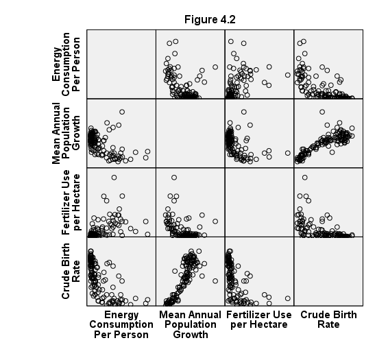
Page 115 Figure 4.2 Scatterplot matrix for data from 122 countries.
GET FILE 'd:nations.sav'.

GGRAPH
  /GRAPHDATASET NAME="graphdataset" VARIABLES=encon85 popgro85 fert84 birthr85
  /GRAPHSPEC SOURCE=INLINE.
BEGIN GPL
  SOURCE: s=userSource(id("graphdataset"))
  DATA: encon85=col(source(s), name("encon85"))
  DATA: popgro85=col(source(s), name("popgro85"))
  DATA: fert84=col(source(s), name("fert84"))
  DATA: birthr85=col(source(s), name("birthr85"))
  GUIDE: text.title( label( "Figure 4.2" ) )
  GUIDE: axis(dim(1.1), ticks(null()))
  GUIDE: axis(dim(2.1), ticks(null()))
  GUIDE: axis(dim(1), gap(0px))
  GUIDE: axis(dim(2), gap(0px))
  TRANS: encon85_label = eval("Energy Consumption Per Person")
  TRANS: popgro85_label = eval("Mean Annual Population Growth")
  TRANS: fert84_label = eval("Fertilizer Use per Hectare")
  TRANS: birthr85_label = eval("Crude Birth Rate")
  ELEMENT: point(position((encon85/encon85_label+popgro85/popgro85_label+fert84/fert84_label+birthr85/birthr85_label)*
(encon85/encon85_label+popgro85/popgro85_label+fert84/fert84_label+birthr85/birthr85_label)))
END GPL.
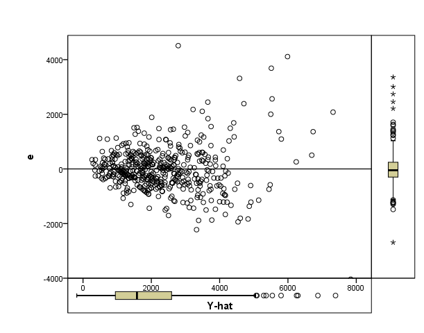
Page 116 Figure 4.3 Residuals (e) versus predicted values (Y-hat) from regression
of 1981 household water use on seven predictors.
GET FILE 'd:concord1.sav'.

REGRESSION
  /DEPENDENT water81
  /METHOD=ENTER income water80 educat retire peop81 cpeop peop80
  /SAVE PRED RESID.
| Model | Variables Entered | Variables Removed | Method |
|---|---|---|---|
| 1 | # people living in 1980, Education in Years, Increase in # of People, head of house retired?, Income in Thousands, Summer 1980 Water Use(a) | . | Enter |
| a Tolerance = .000 limits reached. | |||
| b Dependent Variable: Summer 1981 Water Use | |||
| Model | R | R Square | Adjusted R Square | Std. Error of the Estimate |
|---|---|---|---|---|
| 1 | .823(a) | .677 | .673 | 849.349 |
| a Predictors: (Constant), # people living in 1980, Education in Years, Increase in # of People, head of house retired?, Income in Thousands, Summer 1980 Water Use | ||||
| b Dependent Variable: Summer 1981 Water Use | ||||
| Model | Sum of Squares | df | Mean Square | F | Sig. | |
|---|---|---|---|---|---|---|
| 1 | Regression | 740477522.059 | 6 | 123412920.343 | 171.076 | .000(a) |
| Residual | 352761187.618 | 489 | 721393.022 | |
|
|
| Total | 1093238709.677 | 495 | |
|
|
|
| a Predictors: (Constant), # people living in 1980, Education in Years, Increase in # of People, head of house retired?, Income in Thousands, Summer 1980 Water Use | ||||||
| b Dependent Variable: Summer 1981 Water Use | ||||||
| |
Unstandardized Coefficients | Standardized Coefficients | t | Sig. | ||
|---|---|---|---|---|---|---|
| Model | B | Std. Error | Beta | |||
| 1 | (Constant) | 242.220 | 206.864 | |
1.171 | .242 |
| Income in Thousands | 20.967 | 3.464 | .184 | 6.053 | .000 | |
| Summer 1980 Water Use | .492 | .026 | .584 | 18.671 | .000 | |
| Education in Years | -41.866 | 13.220 | -.087 | -3.167 | .002 | |
| head of house retired? | 189.184 | 95.021 | .058 | 1.991 | .047 | |
| Increase in # of People | 344.651 | 80.806 | .112 | 4.265 | .000 | |
| # people living in 1980 | 248.197 | 28.725 | .277 | 8.641 | .000 | |
| a Dependent Variable: Summer 1981 Water Use | ||||||
| |
Beta In | t | Sig. | Partial Correlation | Collinearity Statistics | |
|---|---|---|---|---|---|---|
| Model | Tolerance | |||||
| 1 | # of People Resident, 1981 | .(a) | . | . | . | .000 |
| a Predictors in the Model: (Constant), # people living in 1980, Education in Years, Increase in # of People, head of house retired?, Income in Thousands, Summer 1980 Water Use | ||||||
| b Dependent Variable: Summer 1981 Water Use | ||||||
| Case Number | Std. Residual | Summer 1981 Water Use |
|---|---|---|
| 79 | 3.020 | 8100 |
| 80 | 5.313 | 7300 |
| 85 | 5.932 | 6500 |
| 94 | -4.753 | 3800 |
| 118 | 3.904 | 7900 |
| 124 | 4.842 | 10100 |
| 125 | 4.341 | 9200 |
| a Dependent Variable: Summer 1981 Water Use | ||
| |
Minimum | Maximum | Mean | Std. Deviation | N |
|---|---|---|---|---|---|
| Predicted Value | 262.78 | 7837.05 | 2298.39 | 1223.076 | 496 |
| Residual | -4037.05 | 5037.99 | .00 | 844.185 | 496 |
| Std. Predicted Value | -1.664 | 4.528 | .000 | 1.000 | 496 |
| Std. Residual | -4.753 | 5.932 | .000 | .994 | 496 |
| a Dependent Variable: Summer 1981 Water Use | |||||
formats pred_1 (f4.0) resid_1 (f5.0).
GGRAPH
  /GRAPHDATASET NAME="graphdataset" VARIABLES=pred_1 resid_1
  /GRAPHSPEC SOURCE=INLINE.
BEGIN GPL
SOURCE: s=userSource(id("graphdataset"))
DATA: pred_1=col(source(s), name("pred_1"))
DATA: resid_1=col(source(s), name("resid_1"))
GRAPH: begin(origin(15.0%, 10.0%), scale(70.0%, 70.0%))
GUIDE: axis( dim( 1 ), label( "Y-hat" ))
GUIDE: axis( dim( 2 ), label( "e" ) )
GUIDE: form.line(position(*, 0))
SCALE: linear( dim( 1 ), min(0), max(8000) )
SCALE: linear( dim( 2 ), min(-4000), max(4000) )
ELEMENT: point(position(pred_1*resid_1))
GRAPH: end()
GRAPH: begin(origin(15.0%, 80.0%), scale(70.0%, 10.0%))
COORD: transpose()
GUIDE: axis(dim(1), ticks(null()))
GUIDE: axis(dim(2), null())
ELEMENT: schema(position(bin.quantile.letter(1*pred_1)))
GRAPH: end()
GRAPH: begin(origin(85.0%, 10.0%), scale(10.0%, 70.0%))
GUIDE: axis(dim(1), ticks(null()))
GUIDE: axis(dim(2), null())
ELEMENT: schema(position(bin.quantile.letter(1*resid_1)))
GRAPH: end()
END GPL.
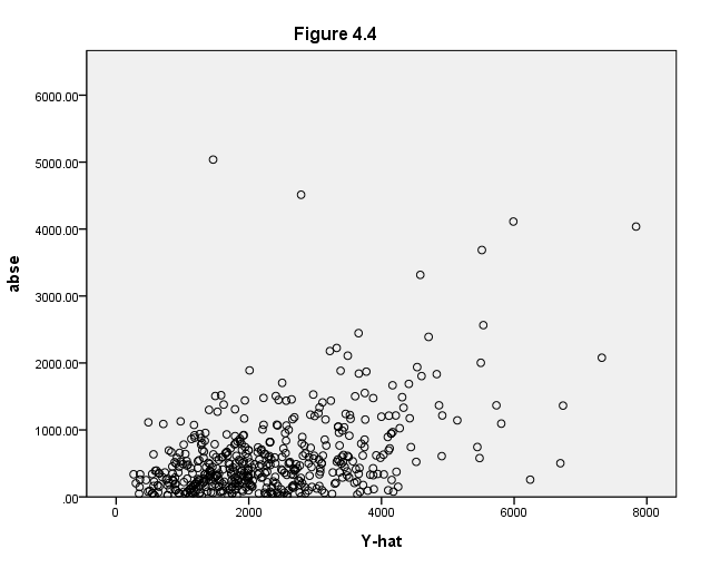
Page 117 Figure 4.4 Absolute residuals |e| versus Y-hat, with band regression line indicating
heteroscedasticity (household water-use regression).
compute abse=abs(res_1).
execute.
NOTE: We do not know how to do band regression in SPSS, so the lines are not included on this graph.
compute abse=abs(resid_1).
execute.
GGRAPH
  /GRAPHDATASET NAME="graphdataset" VARIABLES=pred_1 abse
  /GRAPHSPEC SOURCE=INLINE.
BEGIN GPL
SOURCE: s=userSource(id("graphdataset"))
DATA: pred_1=col(source(s), name("pred_1"))
DATA: abse=col(source(s), name("abse"))
GUIDE: text.title( label( "Figure 4.4" ) )
GUIDE: axis(dim(1), label("Y-hat"))
GUIDE: axis(dim(2), label("abse"))
ELEMENT: point(position(pred_1*abse))
END GPL.
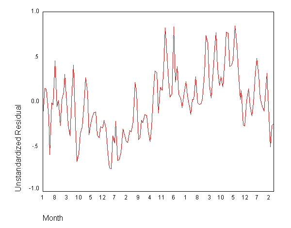
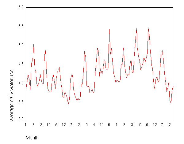
Page 119 Figure 4.5 Time plot of average daily water use by the city of Concord, 1970-1981.
GET FILE 'd:concord2.sav'.

TSPLOT VARIABLES= h2ouse
  /ID= month
  /NOLOG
  /FORMAT NOFILL NOREFERENCE.
MODEL: MOD_4.
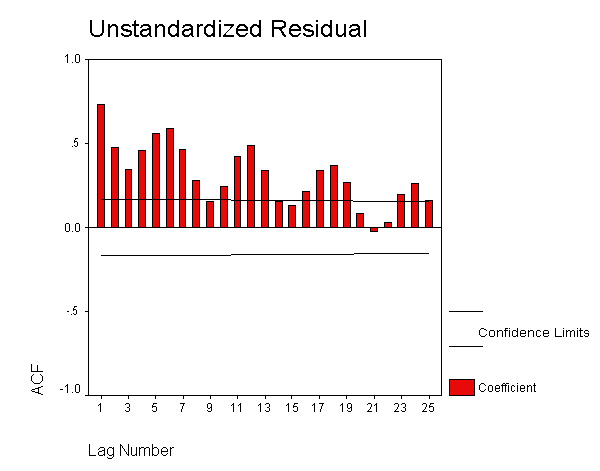
Page 121 Figure 4.6 Correlogram showing autocorrelation of Concord water-use residuals, at monthly lags 0-25.
REGRESSION
  /DEPENDENT h2ouse
  /METHOD=ENTER temp rain educ
  /SAVE RESID.
| Model | Variables Entered | Variables Removed | Method |
|---|---|---|---|
| 1 | conservation campaign dummy, average monthly temperature, precipitation in inches(a) | . | Enter |
| a All requested variables entered. | |||
| b Dependent Variable: average daily water use | |||
| Model | R | R Square | Adjusted R Square | Std. Error of the Estimate |
|---|---|---|---|---|
| 1 | .572(a) | .327 | .312 | .36045 |
| a Predictors: (Constant), conservation campaign dummy, average monthly temperature, precipitation in inches | ||||
| b Dependent Variable: average daily water use | ||||
| Model | Sum of Squares | df | Mean Square | F | Sig. | |
|---|---|---|---|---|---|---|
| 1 | Regression | 8.409 | 3 | 2.803 | 21.574 | .000(a) |
| Residual | 17.280 | 133 | .130 | |
|
|
| Total | 25.689 | 136 | |
|
|
|
| a Predictors: (Constant), conservation campaign dummy, average monthly temperature, precipitation in inches | ||||||
| b Dependent Variable: average daily water use | ||||||
| |
Unstandardized Coefficients | Standardized Coefficients | t | Sig. | ||
|---|---|---|---|---|---|---|
| Model | B | Std. Error | Beta | |||
| 1 | (Constant) | 3.828 | .101 | |
38.035 | .000 |
| average monthly temperature | 1.286E-02 | .002 | .540 | 7.574 | .000 | |
| precipitation in inches | -4.743E-02 | .021 | -.160 | -2.234 | .027 | |
| conservation campaign dummy | -.247 | .113 | -.155 | -2.176 | .031 | |
| a Dependent Variable: average daily water use | ||||||
| |
Minimum | Maximum | Mean | Std. Deviation | N |
|---|---|---|---|---|---|
| Predicted Value | 3.6085 | 4.6821 | 4.2350 | .24866 | 137 |
| Residual | -.7493 | .8434 | .0000 | .35646 | 137 |
| Std. Predicted Value | -2.519 | 1.798 | .000 | 1.000 | 137 |
| Std. Residual | -2.079 | 2.340 | .000 | .989 | 137 |
| a Dependent Variable: average daily water use | |||||
ACF  VARIABLES= res_1
  /MXAUTO 25.
MODEL:  MOD_5.

Autocorrelations:   RES_1   Unstandardized Residual

     Auto- Stand.
Lag  Corr.   Err. -1  -.75  -.5 -.25   0   .25  .5   .75   1   Box-Ljung  Prob.

  1   .730   .085                   .   **.************           74.665   .000
  2   .474   .084                   .   **.******                106.294   .000
  3   .345   .084                   .   **.****                  123.220   .000
  4   .460   .084                   .   **.******                153.457   .000
  5   .559   .083                   .   **.********              198.592   .000
  6   .590   .083                   .   **.*********             249.138   .000
  7   .462   .083                   .   **.******                280.362   .000
  8   .281   .082                   .   **.***                   292.008   .000
  9   .154   .082                   .   ***                      295.533   .000
 10   .240   .082                   .   **.**                    304.149   .000
 11   .424   .081                   .   **.*****                 331.345   .000
 12   .485   .081                   .   **.*******               367.238   .000
 13   .341   .081                   .   **.****                  385.068   .000
 14   .153   .080                   .   ***                      388.689   .000
 15   .130   .080                   .   ***                      391.315   .000
 16   .216   .080                   .   **.*                     398.639   .000
 17   .340   .079                   .   **.****                  416.933   .000
 18   .369   .079                   .   **.****                  438.779   .000
 19   .272   .079                   .   **.**                    450.690   .000
 20   .086   .078                   .   **.                      451.881   .000
 21  -.019   .078                   .  *  .                      451.940   .000
 22   .029   .078                   .   * .                      452.082   .000
 23   .198   .077                   .   **.*                     458.645   .000
 24   .261   .077                   .   **.**                    470.114   .000
 25   .162   .077                   .   ***                      474.561   .000

Plot Symbols:      Autocorrelations *     Two Standard Error Limits .

Total cases:  137     Computable first lags:  136
Page 122 Figure 4.7 Time plot of concord water-use residuals.
TSPLOT VARIABLES= res_1
  /ID= month.
MODEL: MOD_6.
Page 122 Figure 4.8 Time plots of Concord water-use residuals, showing effects of repeated smoothing by running means of span 3.
NOTE: We do not know how smooth by running means.
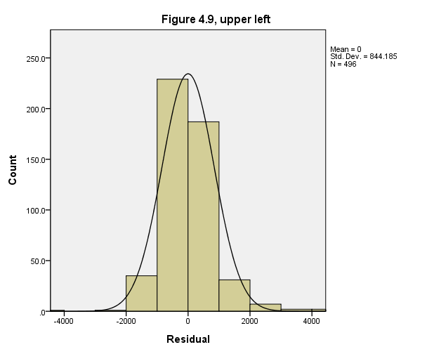
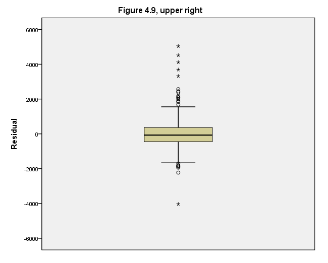
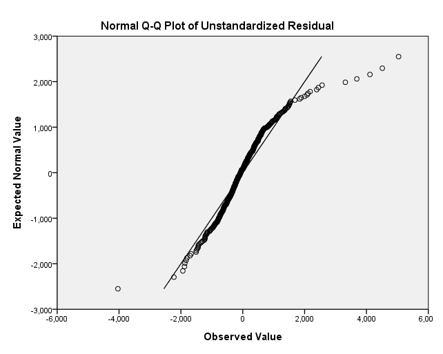
Page 124 Figure 4.9 Four views showing nonnormality of residuals from regression of 1981 household water use on six predictors.
GET FILE 'd:concord1.sav'.

REGRESSION
  /DEPENDENT water81
  /METHOD=ENTER income water80 educat retire peop81 cpeop
  /SAVE RESID.
| Model | Variables Entered | Variables Removed | Method |
|---|---|---|---|
| 1 | Increase in # of People, Education in Years, Summer 1980 Water Use, head of house retired?, Income in Thousands, # of People Resident, 1981(a) | . | Enter |
| a All requested variables entered. | |||
| b Dependent Variable: Summer 1981 Water Use | |||
| Model | R | R Square | Adjusted R Square | Std. Error of the Estimate |
|---|---|---|---|---|
| 1 | .823(a) | .677 | .673 | 849.349 |
| a Predictors: (Constant), Increase in # of People, Education in Years, Summer 1980 Water Use, head of house retired?, Income in Thousands, # of People Resident, 1981 | ||||
| b Dependent Variable: Summer 1981 Water Use | ||||
| Model | Sum of Squares | df | Mean Square | F | Sig. | |
|---|---|---|---|---|---|---|
| 1 | Regression | 740477522.059 | 6 | 123412920.343 | 171.076 | .000(a) |
| Residual | 352761187.618 | 489 | 721393.022 | |
|
|
| Total | 1093238709.677 | 495 | |
|
|
|
| a Predictors: (Constant), Increase in # of People, Education in Years, Summer 1980 Water Use, head of house retired?, Income in Thousands, # of People Resident, 1981 | ||||||
| b Dependent Variable: Summer 1981 Water Use | ||||||
| |
Unstandardized Coefficients | Standardized Coefficients | t | Sig. | ||
|---|---|---|---|---|---|---|
| Model | B | Std. Error | Beta | |||
| 1 | (Constant) | 242.220 | 206.864 | |
1.171 | .242 |
| Income in Thousands | 20.967 | 3.464 | .184 | 6.053 | .000 | |
| Summer 1980 Water Use | .492 | .026 | .584 | 18.671 | .000 | |
| Education in Years | -41.866 | 13.220 | -.087 | -3.167 | .002 | |
| head of house retired? | 189.184 | 95.021 | .058 | 1.991 | .047 | |
| # of People Resident, 1981 | 248.197 | 28.725 | .277 | 8.641 | .000 | |
| Increase in # of People | 96.454 | 80.519 | .031 | 1.198 | .232 | |
| a Dependent Variable: Summer 1981 Water Use | ||||||
| Case Number | Std. Residual | Summer 1981 Water Use |
|---|---|---|
| 79 | 3.020 | 8100 |
| 80 | 5.313 | 7300 |
| 85 | 5.932 | 6500 |
| 94 | -4.753 | 3800 |
| 118 | 3.904 | 7900 |
| 124 | 4.842 | 10100 |
| 125 | 4.341 | 9200 |
| a Dependent Variable: Summer 1981 Water Use | ||
| |
Minimum | Maximum | Mean | Std. Deviation | N |
|---|---|---|---|---|---|
| Predicted Value | 262.78 | 7837.05 | 2298.39 | 1223.076 | 496 |
| Residual | -4037.05 | 5037.99 | .00 | 844.185 | 496 |
| Std. Predicted Value | -1.664 | 4.528 | .000 | 1.000 | 496 |
| Std. Residual | -4.753 | 5.932 | .000 | .994 | 496 |
| a Dependent Variable: Summer 1981 Water Use | |||||
Upper left panel of Figure 4.9
formats resid_1 pred_1 (f5.0).
GGRAPH
  /GRAPHDATASET NAME="GraphDataset" VARIABLES= resid_1
  /GRAPHSPEC SOURCE=INLINE .
BEGIN GPL
SOURCE: s=userSource( id( "GraphDataset" ) )
DATA: Y_Var=col( source(s), name( "$count" ) )
DATA: resid_1=col( source(s), name( "resid_1" ) )
GUIDE: text.title( label( "Figure 4.9, upper left" ) )
GUIDE: axis( dim( 1 ), label( "Residual" ), delta(2000) )
GUIDE: axis( dim( 2 ), label( "Count" ) )
SCALE: linear( dim( 1 ), min(-4000), max(4000) )
ELEMENT: interval( position( summary.count( bin.rect( resid_1, binStart( 0 ), binCount( 13 ) ) ) ) )
ELEMENT: line( position( density.normal( resid_1 ) ) )
END GPL.
Upper right panel of Figure 4.9
GGRAPH
  /GRAPHDATASET NAME="graphdataset" VARIABLES=resid_1
  /GRAPHSPEC SOURCE=INLINE.
BEGIN GPL
SOURCE: s=userSource(id("graphdataset"))
DATA: resid_1=col(source(s), name("resid_1"))
GUIDE: text.title( label( "Figure 4.9, upper right" ))
COORD: rect(dim(1), transpose())
GUIDE: axis(dim(1), label("Residual"), delta(2000))
SCALE: linear( dim( 2 ), min(-4000), max(4000) )
ELEMENT: schema(position(bin.quantile.letter(resid_1)))
END GPL.
Lower left panel of Figure 4.9
NOTE: We do not know how to make a symmetry plot in SPSS.
Lower right panel of Figure 4.9
pplot
/variable = resid_1
/type q-q.
Page 127 Table 4.3 Summary statistics for DFBETAS of coefficients in household water-use regression
of Equation [4.3].
REGRESSION
  /DEPENDENT water81
  /METHOD=ENTER income water80 educat retire peop81 cpeop
  /SAVE DFBETA.
| Model | Variables Entered | Variables Removed | Method |
|---|---|---|---|
| 1 | Increase in # of People, Education in Years, Summer 1980 Water Use, head of house retired?, Income in Thousands, # of People Resident, 1981(a) | . | Enter |
| a All requested variables entered. | |||
| b Dependent Variable: Summer 1981 Water Use | |||
| Model | R | R Square | Adjusted R Square | Std. Error of the Estimate |
|---|---|---|---|---|
| 1 | .823(a) | .677 | .673 | 849.349 |
| a Predictors: (Constant), Increase in # of People, Education in Years, Summer 1980 Water Use, head of house retired?, Income in Thousands, # of People Resident, 1981 | ||||
| b Dependent Variable: Summer 1981 Water Use | ||||
| Model | Sum of Squares | df | Mean Square | F | Sig. | |
|---|---|---|---|---|---|---|
| 1 | Regression | 740477522.059 | 6 | 123412920.343 | 171.076 | .000(a) |
| Residual | 352761187.618 | 489 | 721393.022 | |
|
|
| Total | 1093238709.677 | 495 | |
|
|
|
| a Predictors: (Constant), Increase in # of People, Education in Years, Summer 1980 Water Use, head of house retired?, Income in Thousands, # of People Resident, 1981 | ||||||
| b Dependent Variable: Summer 1981 Water Use | ||||||
| |
Unstandardized Coefficients | Standardized Coefficients | t | Sig. | ||
|---|---|---|---|---|---|---|
| Model | B | Std. Error | Beta | |||
| 1 | (Constant) | 242.220 | 206.864 | |
1.171 | .242 |
| Income in Thousands | 20.967 | 3.464 | .184 | 6.053 | .000 | |
| Summer 1980 Water Use | .492 | .026 | .584 | 18.671 | .000 | |
| Education in Years | -41.866 | 13.220 | -.087 | -3.167 | .002 | |
| head of house retired? | 189.184 | 95.021 | .058 | 1.991 | .047 | |
| # of People Resident, 1981 | 248.197 | 28.725 | .277 | 8.641 | .000 | |
| Increase in # of People | 96.454 | 80.519 | .031 | 1.198 | .232 | |
| a Dependent Variable: Summer 1981 Water Use | ||||||
| Case Number | Std. Residual | Summer 1981 Water Use |
|---|---|---|
| 79 | 3.020 | 8100 |
| 80 | 5.313 | 7300 |
| 85 | 5.932 | 6500 |
| 94 | -4.753 | 3800 |
| 118 | 3.904 | 7900 |
| 124 | 4.842 | 10100 |
| 125 | 4.341 | 9200 |
| a Dependent Variable: Summer 1981 Water Use | ||
| |
Minimum | Maximum | Mean | Std. Deviation | N |
|---|---|---|---|---|---|
| Predicted Value | 262.78 | 7837.05 | 2298.39 | 1223.076 | 496 |
| Std. Predicted Value | -1.664 | 4.528 | .000 | 1.000 | 496 |
| Standard Error of Predicted Value | 48.840 | 273.580 | 95.681 | 32.066 | 496 |
| Adjusted Predicted Value | 256.12 | 8196.38 | 2297.98 | 1222.737 | 496 |
| Residual | -4037.05 | 5037.99 | .00 | 844.185 | 496 |
| Std. Residual | -4.753 | 5.932 | .000 | .994 | 496 |
| Stud. Residual | -4.960 | 5.966 | .000 | 1.007 | 496 |
| Deleted Residual | -4396.38 | 5095.83 | .41 | 866.178 | 496 |
| Stud. Deleted Residual | -5.085 | 6.189 | .002 | 1.016 | 496 |
| Mahal. Distance | .639 | 50.359 | 5.988 | 5.710 | 496 |
| Cook’s Distance | .000 | .313 | .004 | .021 | 496 |
| Centered Leverage Value | .001 | .102 | .012 | .012 | 496 |
| a Dependent Variable: Summer 1981 Water Use | |||||
DESCRIPTIVES VARIABLES=dfb1_1 dfb2_1 dfb3_1 dfb4_1 dfb5_1 dfb6_1
  /STATISTICS=MEAN STDDEV MIN MAX.
| |
N | Minimum | Maximum | Mean | Std. Deviation |
|---|---|---|---|---|---|
| DFBETA INCOME | 496 | -.85919 | 4.54791 | .0010205 | .30944938 |
| DFBETA WATER80 | 496 | -.03567 | .01760 | -.0000037 | .00231794 |
| DFBETA EDUCAT | 496 | -4.64425 | 1.34235 | -.0017557 | .56819471 |
| DFBETA RETIRE | 496 | -19.84839 | 26.33657 | .0058540 | 4.20308173 |
| DFBETA PEOP81 | 496 | -11.99661 | 12.76215 | .0016764 | 1.74564279 |
| DFBETA CPEOP | 496 | -18.80571 | 28.17114 | -.0031481 | 3.26555664 |
| Valid N (listwise) | 496 | |
|
|
|
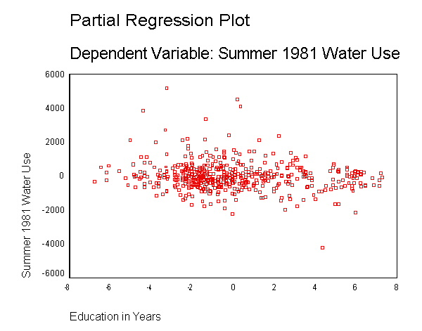
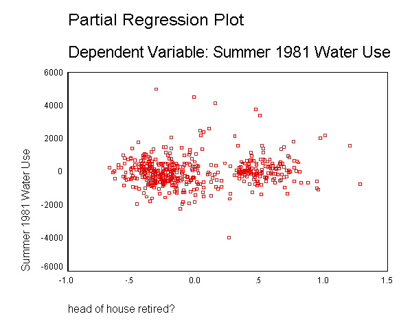
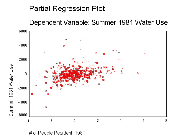
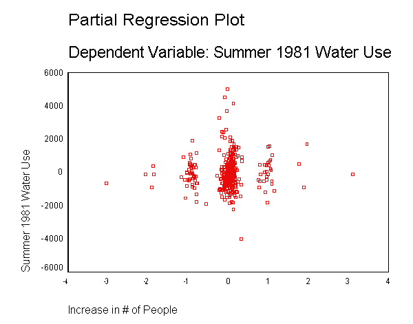
Page 127 Figure 4.10 Leverage plot of 1981 household water use versus income, adjusting for other predictors.
REGRESSION
  /DEPENDENT water81
  /METHOD=ENTER income water80 educat retire peop81 cpeop
  /PARTIALPLOT ALL.
| Model | Variables Entered | Variables Removed | Method |
|---|---|---|---|
| 1 | Increase in # of People, Education in Years, Summer 1980 Water Use, head of house retired?, Income in Thousands, # of People Resident, 1981(a) | . | Enter |
| a All requested variables entered. | |||
| b Dependent Variable: Summer 1981 Water Use | |||
| Model | R | R Square | Adjusted R Square | Std. Error of the Estimate |
|---|---|---|---|---|
| 1 | .823(a) | .677 | .673 | 849.349 |
| a Predictors: (Constant), Increase in # of People, Education in Years, Summer 1980 Water Use, head of house retired?, Income in Thousands, # of People Resident, 1981 | ||||
| b Dependent Variable: Summer 1981 Water Use | ||||
| Model | Sum of Squares | df | Mean Square | F | Sig. | |
|---|---|---|---|---|---|---|
| 1 | Regression | 740477522.059 | 6 | 123412920.343 | 171.076 | .000(a) |
| Residual | 352761187.618 | 489 | 721393.022 | |
|
|
| Total | 1093238709.677 | 495 | |
|
|
|
| a Predictors: (Constant), Increase in # of People, Education in Years, Summer 1980 Water Use, head of house retired?, Income in Thousands, # of People Resident, 1981 | ||||||
| b Dependent Variable: Summer 1981 Water Use | ||||||
| |
Unstandardized Coefficients | Standardized Coefficients | t | Sig. | ||
|---|---|---|---|---|---|---|
| Model | B | Std. Error | Beta | |||
| 1 | (Constant) | 242.220 | 206.864 | |
1.171 | .242 |
| Income in Thousands | 20.967 | 3.464 | .184 | 6.053 | .000 | |
| Summer 1980 Water Use | .492 | .026 | .584 | 18.671 | .000 | |
| Education in Years | -41.866 | 13.220 | -.087 | -3.167 | .002 | |
| head of house retired? | 189.184 | 95.021 | .058 | 1.991 | .047 | |
| # of People Resident, 1981 | 248.197 | 28.725 | .277 | 8.641 | .000 | |
| Increase in # of People | 96.454 | 80.519 | .031 | 1.198 | .232 | |
| a Dependent Variable: Summer 1981 Water Use | ||||||
| Case Number | Std. Residual | Summer 1981 Water Use |
|---|---|---|
| 79 | 3.020 | 8100 |
| 80 | 5.313 | 7300 |
| 85 | 5.932 | 6500 |
| 94 | -4.753 | 3800 |
| 118 | 3.904 | 7900 |
| 124 | 4.842 | 10100 |
| 125 | 4.341 | 9200 |
| a Dependent Variable: Summer 1981 Water Use | ||
| |
Minimum | Maximum | Mean | Std. Deviation | N |
|---|---|---|---|---|---|
| Predicted Value | 262.78 | 7837.05 | 2298.39 | 1223.076 | 496 |
| Residual | -4037.05 | 5037.99 | .00 | 844.185 | 496 |
| Std. Predicted Value | -1.664 | 4.528 | .000 | 1.000 | 496 |
| Std. Residual | -4.753 | 5.932 | .000 | .994 | 496 |
| a Dependent Variable: Summer 1981 Water Use | |||||
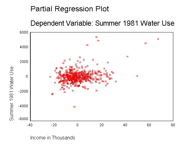
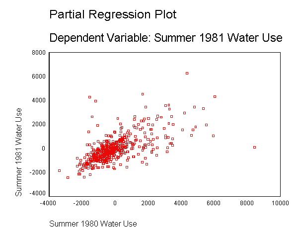
Page 128 Figure 4.11 Proportional leverage plot (symbols proportional to DFBETAS)
of 1981 household water use versus income, adjusting for five other predictors.NOTE: This syntax for this graph is the same as above. The only difference between
the two graphs is the use of the symbols proportional to DFBETAS, and SPSS does not
allow you to make the symbols proportional on this type of graph.Page 129 Figure 4.12 Proportional leverage plot of 1981 household water use versus
1980 water use, adjusting for five other predictors.NOTE: The syntax for this graph is the same as for Figure 4.10, as SPSS gives you all
of the possible leverage plots.Page 129 Figure 4.13 Proportional leverage plots of 1981 household water use versus X,
each adjusting for five other predictors.NOTE: The syntax for this graph is the same as for Figure 4.10, as SPSS gives you all
of the possible leverage plots.
Page 133 Table 4.4 Case statistics for three influential households (see Figures 4.11 and 4.12).
REGRESSION
 /DEPENDENT water81
 /METHOD=ENTER income water80 educat retire peop81 cpeop
 /SAVE COOK LEVER RESID ZRESID SRESID DFBETA.
| Model | Variables Entered | Variables Removed | Method |
|---|---|---|---|
| 1 | Increase in # of People, Education in Years, Summer 1980 Water Use, head of house retired?, Income in Thousands, # of People Resident, 1981(a) | . | Enter |
| a All requested variables entered. | |||
| b Dependent Variable: Summer 1981 Water Use | |||
| Model | R | R Square | Adjusted R Square | Std. Error of the Estimate |
|---|---|---|---|---|
| 1 | .823(a) | .677 | .673 | 849.349 |
| a Predictors: (Constant), Increase in # of People, Education in Years, Summer 1980 Water Use, head of house retired?, Income in Thousands, # of People Resident, 1981 | ||||
| b Dependent Variable: Summer 1981 Water Use | ||||
| Model | Sum of Squares | df | Mean Square | F | Sig. | |
|---|---|---|---|---|---|---|
| 1 | Regression | 740477522.059 | 6 | 123412920.343 | 171.076 | .000(a) |
| Residual | 352761187.618 | 489 | 721393.022 | |
|
|
| Total | 1093238709.677 | 495 | |
|
|
|
| a Predictors: (Constant), Increase in # of People, Education in Years, Summer 1980 Water Use, head of house retired?, Income in Thousands, # of People Resident, 1981 | ||||||
| b Dependent Variable: Summer 1981 Water Use | ||||||
| |
Unstandardized Coefficients | Standardized Coefficients | t | Sig. | ||
|---|---|---|---|---|---|---|
| Model | B | Std. Error | Beta | |||
| 1 | (Constant) | 242.220 | 206.864 | |
1.171 | .242 |
| Income in Thousands | 20.967 | 3.464 | .184 | 6.053 | .000 | |
| Summer 1980 Water Use | .492 | .026 | .584 | 18.671 | .000 | |
| Education in Years | -41.866 | 13.220 | -.087 | -3.167 | .002 | |
| head of house retired? | 189.184 | 95.021 | .058 | 1.991 | .047 | |
| # of People Resident, 1981 | 248.197 | 28.725 | .277 | 8.641 | .000 | |
| Increase in # of People | 96.454 | 80.519 | .031 | 1.198 | .232 | |
| a Dependent Variable: Summer 1981 Water Use | ||||||
| Case Number | Std. Residual | Summer 1981 Water Use |
|---|---|---|
| 79 | 3.020 | 8100 |
| 80 | 5.313 | 7300 |
| 85 | 5.932 | 6500 |
| 94 | -4.753 | 3800 |
| 118 | 3.904 | 7900 |
| 124 | 4.842 | 10100 |
| 125 | 4.341 | 9200 |
| a Dependent Variable: Summer 1981 Water Use | ||
| |
Minimum | Maximum | Mean | Std. Deviation | N |
|---|---|---|---|---|---|
| Predicted Value | 262.78 | 7837.05 | 2298.39 | 1223.076 | 496 |
| Std. Predicted Value | -1.664 | 4.528 | .000 | 1.000 | 496 |
| Standard Error of Predicted Value | 48.840 | 273.580 | 95.681 | 32.066 | 496 |
| Adjusted Predicted Value | 256.12 | 8196.38 | 2297.98 | 1222.737 | 496 |
| Residual | -4037.05 | 5037.99 | .00 | 844.185 | 496 |
| Std. Residual | -4.753 | 5.932 | .000 | .994 | 496 |
| Stud. Residual | -4.960 | 5.966 | .000 | 1.007 | 496 |
| Deleted Residual | -4396.38 | 5095.83 | .41 | 866.178 | 496 |
| Stud. Deleted Residual | -5.085 | 6.189 | .002 | 1.016 | 496 |
| Mahal. Distance | .639 | 50.359 | 5.988 | 5.710 | 496 |
| Cook’s Distance | .000 | .313 | .004 | .021 | 496 |
| Centered Leverage Value | .001 | .102 | .012 | .012 | 496 |
| a Dependent Variable: Summer 1981 Water Use | |||||
USE ALL.
COMPUTE filter_$=(case = 101 | case=127 | case=134).
VARIABLE LABEL filter_$ 'case = 101 | case=127 | case=134 (FILTER)'.
VALUE LABELS filter_$  0 'Not Selected' 1 'Selected'.
FILTER BY filter_$.
EXECUTE.

list case res_1 lev_1 zre_1 sre_1 coo_1 dfb1_1 dfb2_1.
The variables are listed in the following order:

LINE   1: CASE RES_1 LEV_1 ZRE_1 SRE_1 COO_1

LINE   2: DFB1_1 DFB2_1


    CASE: 101 -4037.04714   .07972   -4.75311   -4.96013   .31284    .21282    -.03567

    CASE: 127  3315.58478   .05959   3.90368     4.02979   .15232   3.34230    -.00469

    CASE: 134  3687.11597   .08836   4.34111     4.55167   .29407   4.54791     .00648


Number of cases read:  3    Number of cases listed:  3
Page 134 Table 4.5 Checking for multicollinearlity: tolerances of X variables in water-use regression [4.3].
FILTER OFF.
REGRESSION
  /statistics=tol
  /DEPENDENT water81
  /METHOD=ENTER income water80 educat retire peop81 cpeop.
| Model | Variables Entered | Variables Removed | Method |
|---|---|---|---|
| 1 | Increase in # of People, Education in Years, Summer 1980 Water Use, head of house retired?, Income in Thousands, # of People Resident, 1981(a) | . | Enter |
| a All requested variables entered. | |||
| b Dependent Variable: Summer 1981 Water Use | |||
| |
Collinearity Statistics | ||
|---|---|---|---|
| Model | Tolerance | VIF | |
| 1 | Income in Thousands | .712 | 1.404 |
| Summer 1980 Water Use | .675 | 1.482 | |
| Education in Years | .873 | 1.145 | |
| head of house retired? | .776 | 1.289 | |
| # of People Resident, 1981 | .643 | 1.555 | |
| Increase in # of People | .957 | 1.045 | |
| a Dependent Variable: Summer 1981 Water Use | |||

