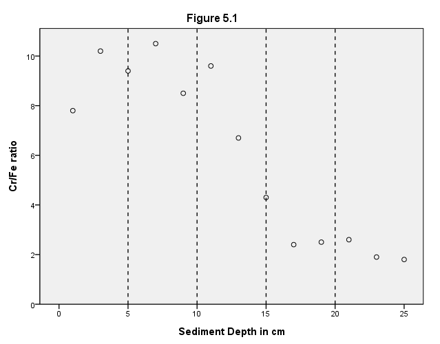
Regression with Graphics by Lawrence Hamilton Chapter 5: Fitting curves

Page 146 Figure 5.1 Exploratory band regression curve (5 bands) based on cross-medians from Table 5.1.

GET FILE 'd:rwgdatacrfe.sav'.

NOTE: We were unable to add the band lines as shown in the text.

formats crfe (f2.0).
GGRAPH
  /GRAPHDATASET NAME="graphdataset" VARIABLES=depth crfe
  /GRAPHSPEC SOURCE=INLINE.
BEGIN GPL
SOURCE: s=userSource(id("graphdataset"))
DATA: depth=col(source(s), name("depth"))
DATA: crfe=col(source(s), name("crfe"))
GUIDE: text.title( label( "Figure 5.1" ) )
GUIDE: axis(dim(1), label("Sediment Depth in cm"), delta(5))
GUIDE: axis(dim(2), label("Cr/Fe ratio"), delta(2))
GUIDE: form.line(position(5), shape(shape.dash))
GUIDE: form.line(position(10), shape(shape.dash))
GUIDE: form.line(position(15), shape(shape.dash))
GUIDE: form.line(position(20), shape(shape.dash))
SCALE: linear(dim(1), min(0), max(25))
SCALE: linear(dim(2), min(0), max(10))
ELEMENT: point(position(depth*crfe))
END GPL.

Page 147 Table 5.1 Cross-medians for exploratory regression with five bands; ratio of chromium (Cr) to iron (Fe) in Great Bay sediments.

NOTE: You need to add a column called case in which you just list the numbers from 1 to 13. After you get the medians from the examine command below, you need to put them into columns in the data set.

GET  FILE 'd:appsrwgdatacrfe1.sav'.

EXAMINE
  VARIABLES=crfe depth BY band
  /PLOT NONE
  /PERCENTILES(50)
  /STATISTICS NONE
  /NOTOTAL.

**Case Processing Summary**
		Cases
		Valid		Missing		Total
	BAND	N	Percent	N	Percent	N	Percent
Cr/Fe ratio	1.00	2	100.0%	0	.0%	2	100.0%
	2.00	3	100.0%	0	.0%	3	100.0%
	3.00	2	100.0%	0	.0%	2	100.0%
	4.00	3	100.0%	0	.0%	3	100.0%
	5.00	3	100.0%	0	.0%	3	100.0%
Depth in cm	1.00	2	100.0%	0	.0%	2	100.0%
	2.00	3	100.0%	0	.0%	3	100.0%
	3.00	2	100.0%	0	.0%	2	100.0%
	4.00	3	100.0%	0	.0%	3	100.0%
	5.00	3	100.0%	0	.0%	3	100.0%

**Percentiles**
			Percentiles
	BAND	50
Weighted Average(Definition 1)	Cr/Fe ratio	1.00	9.0000
		2.00	9.4000
		3.00	8.1500
		4.00	2.5000
		5.00	1.9000
	Depth in cm	1.00	2.00
		2.00	7.00
		3.00	12.00
		4.00	17.00
		5.00	23.00
Tukey’s Hinges	Cr/Fe ratio	1.00	9.0000
		2.00	9.4000
		3.00	8.1500
		4.00	2.5000
		5.00	1.9000
	Depth in cm	1.00	2.00
		2.00	7.00
		3.00	12.00
		4.00	17.00
		5.00	23.00

list case depth crfe medianx mediany.

    CASE    DEPTH      CRFE  MEDIANX  MEDIANY

    1.00        1      7.80     2.00     9.00
    2.00        3     10.20     2.00     9.00
    3.00        5      9.40     7.00     9.40
    4.00        7     10.50     7.00     9.40
    5.00        9      8.50     7.00     9.40
    6.00       11      9.60    12.00     8.15
    7.00       13      6.70    12.00     8.15
    8.00       15      4.30    12.00     2.50
    9.00       17      2.40    17.00     2.50
   10.00       19      2.50    17.00     2.50
   11.00       21      2.60    23.00     1.90
   12.00       23      1.90    23.00     1.90
   13.00       25      1.80    23.00     1.90

Number of cases read:  13    Number of cases listed:  13

Page 155 Table 5.2 Curvilinear regression – water-use regression with transformed variables.

GET FILE 'd:appsrwgdataconcord1.sav'.

compute y=water81**.3.
compute x1=income**.3.
compute x2=water80**.3.
compute x5=ln(peop81).
compute x7=ln(peop81/peop80).
execute.

REGRESSION
  /DEPENDENT y
  /METHOD=ENTER x1 x2 x5 x7 educat retire.

**Variables Entered/Removed(b)**
Model	Variables Entered	Variables Removed	Method
1	head of house retired?, X7, Education in Years, X2, X1, X5(a)	.	Enter
a All requested variables entered.
b Dependent Variable: Y

**Model Summary**
Model	R	R Square	Adjusted R Square	Std. Error of the Estimate
1	.848(a)	.720	.717	1.02088
a Predictors: (Constant), head of house retired?, X7, Education in Years, X2, X1, X5

**ANOVA(b)**
Model		Sum of Squares	df	Mean Square	F	Sig.
1	Regression	1310.117	6	218.353	209.511	.000(a)
	Residual	509.637	489	1.042
	Total	1819.754	495
a Predictors: (Constant), head of house retired?, X7, Education in Years, X2, X1, X5
b Dependent Variable: Y

**Coefficients(a)**
		Unstandardized Coefficients		Standardized Coefficients	t	Sig.
Model		B	Std. Error	Beta	t	Sig.
1	(Constant)	1.856	.385		4.822	.000
	X1	.516	.130	.120	3.976	.000
	X2	.626	.029	.656	21.508	.000
	X5	.715	.110	.208	6.469	.000
	X7	.916	.263	.087	3.485	.001
	Education in Years	-3.613E-02	.016	-.058	-2.257	.024
	head of house retired?	.101	.119	.024	.852	.395
a Dependent Variable: Y

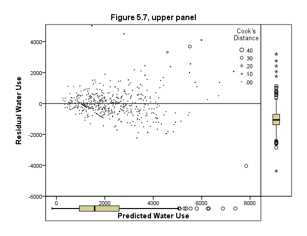
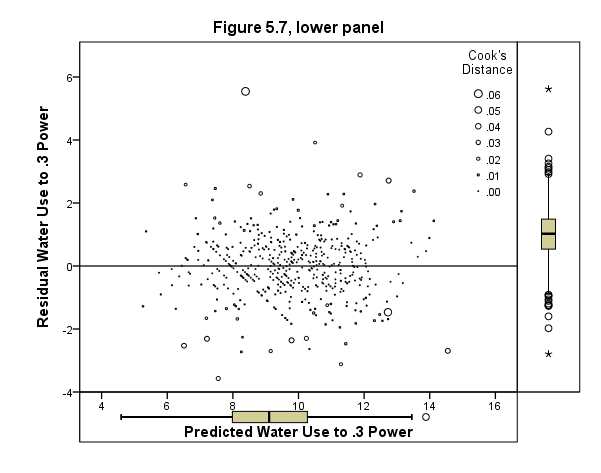
Page 156 Figure 5.7 e-versus-Y-hat plots with points proportional to scaled Cook’s D, for raw-data (top) and transformed-variables (bottom) regression.

Top graph

REGRESSION
   /DEPENDENT water81
  /METHOD=ENTER water80 income educat retire peop81 cpeop
  /SAVE PRED RESID.

**Variables Entered/Removed(b)**
Model	Variables Entered	Variables Removed	Method
1	Increase in # of People, Education in Years, Summer 1980 Water Use, head of house retired?, Income in Thousands, # of People Resident, 1981(a)	.	Enter
a All requested variables entered.
b Dependent Variable: Summer 1981 Water Use

**Model Summary(b)**
Model	R	R Square	Adjusted R Square	Std. Error of the Estimate
1	.823(a)	.677	.673	849.349
a Predictors: (Constant), Increase in # of People, Education in Years, Summer 1980 Water Use, head of house retired?, Income in Thousands, # of People Resident, 1981
b Dependent Variable: Summer 1981 Water Use

**ANOVA(b)**
Model		Sum of Squares	df	Mean Square	F	Sig.
1	Regression	740477522.059	6	123412920.343	171.076	.000(a)
	Residual	352761187.618	489	721393.022
	Total	1093238709.677	495
a Predictors: (Constant), Increase in # of People, Education in Years, Summer 1980 Water Use, head of house retired?, Income in Thousands, # of People Resident, 1981
b Dependent Variable: Summer 1981 Water Use

**Coefficients(a)**
		Unstandardized Coefficients		Standardized Coefficients	t	Sig.
Model		B	Std. Error	Beta	t	Sig.
1	(Constant)	242.220	206.864		1.171	.242
	Summer 1980 Water Use	.492	.026	.584	18.671	.000
	Income in Thousands	20.967	3.464	.184	6.053	.000
	Education in Years	-41.866	13.220	-.087	-3.167	.002
	head of house retired?	189.184	95.021	.058	1.991	.047
	# of People Resident, 1981	248.197	28.725	.277	8.641	.000
	Increase in # of People	96.454	80.519	.031	1.198	.232
a Dependent Variable: Summer 1981 Water Use

**Casewise Diagnostics(a)**
Case Number	Std. Residual	Summer 1981 Water Use
79	3.020	8100
80	5.313	7300
85	5.932	6500
94	-4.753	3800
118	3.904	7900
124	4.842	10100
125	4.341	9200
a Dependent Variable: Summer 1981 Water Use

**Residuals Statistics(a)**
	Minimum	Maximum	Mean	Std. Deviation	N
Predicted Value	262.78	7837.05	2298.39	1223.076	496
Residual	-4037.05	5037.99	.00	844.185	496
Std. Predicted Value	-1.664	4.528	.000	1.000	496
Std. Residual	-4.753	5.932	.000	.994	496
a Dependent Variable: Summer 1981 Water Use


formats pred1 resid1 (f5.0) cook1 (f4.2).
GGRAPH
  /GRAPHDATASET NAME="graphdataset" VARIABLES=pred1 resid1 cook1
  /GRAPHSPEC SOURCE=INLINE.
BEGIN GPL
SOURCE: s=userSource(id("graphdataset"))
DATA: pred1=col(source(s), name("pred1"))
DATA: resid1=col(source(s), name("resid1"))
DATA: cook1=col(source(s), name("cook1"))
GRAPH: begin(origin(15.0%, 10.0%), scale(70.0%, 70.0%))
GUIDE: text.title( label( "Figure 5.7, upper panel" ) )
GUIDE: axis(dim(1), delta(2000), label("Predicted Water Use"))
GUIDE: axis(dim(2), delta(2000), label("Residual Water Use"))
GUIDE: legend(aesthetic(aesthetic.size), label("Cook's Distance"))
GUIDE: form.line(position(*, 0))
SCALE: linear(dim(1), min(0), max(8000))
SCALE: linear(dim(2), min(-6000), max(4000))
ELEMENT: point(position(pred1*resid1), size(cook1))
GRAPH: end()
GRAPH: begin(origin(15.0%, 80.0%), scale(70.0%, 10.0%))
COORD: transpose()
GUIDE: axis(dim(1), ticks(null()))
GUIDE: axis(dim(2), null())
ELEMENT: schema(position(bin.quantile.letter(1*pred1)))
GRAPH: end()
GRAPH: begin(origin(85.0%, 10.0%), scale(10.0%, 70.0%))
GUIDE: axis(dim(1), ticks(null()))
GUIDE: axis(dim(2), null())
ELEMENT: schema(position(bin.quantile.letter(1*resid1)))
GRAPH: end()
END GPL.

Bottom graph

REGRESSION
 /DEPENDENT y
 /METHOD=ENTER x1 x2 x5 x7 educat retire
 /SAVE PRED RESID.

**Variables Entered/Removed(b)**
Model	Variables Entered	Variables Removed	Method
1	head of house retired?, X7, Education in Years, X2, X1, X5(a)	.	Enter
a All requested variables entered.
b Dependent Variable: Y

**Model Summary(b)**
Model	R	R Square	Adjusted R Square	Std. Error of the Estimate
1	.848(a)	.720	.717	1.02088
a Predictors: (Constant), head of house retired?, X7, Education in Years, X2, X1, X5
b Dependent Variable: Y

**ANOVA(b)**
Model		Sum of Squares	df	Mean Square	F	Sig.
1	Regression	1310.117	6	218.353	209.511	.000(a)
	Residual	509.637	489	1.042
	Total	1819.754	495
a Predictors: (Constant), head of house retired?, X7, Education in Years, X2, X1, X5
b Dependent Variable: Y

**Coefficients(a)**
		Unstandardized Coefficients		Standardized Coefficients	t	Sig.
Model		B	Std. Error	Beta	t	Sig.
1	(Constant)	1.856	.385		4.822	.000
	X1	.516	.130	.120	3.976	.000
	X2	.626	.029	.656	21.508	.000
	X5	.715	.110	.208	6.469	.000
	X7	.916	.263	.087	3.485	.001
	Education in Years	-3.613E-02	.016	-.058	-2.257	.024
	head of house retired?	.101	.119	.024	.852	.395
a Dependent Variable: Y

**Casewise Diagnostics(a)**
Case Number	Std. Residual	Y
80	3.838	14.42
85	5.429	13.93
105	-3.499	3.98
175	-4.458	3.98
494	-3.056	8.17
a Dependent Variable: Y

**Residuals Statistics(a)**
	Minimum	Maximum	Mean	Std. Deviation	N
Predicted Value	5.2609	14.5501	9.7770	1.62687	496
Residual	-4.5512	5.5425	.0000	1.01468	496
Std. Predicted Value	-2.776	2.934	.000	1.000	496
Std. Residual	-4.458	5.429	.000	.994	496
a Dependent Variable: Y


formats pred2 resid2 (f5.0) cook2 (f4.2).
GGRAPH
  /GRAPHDATASET NAME="graphdataset" VARIABLES=pred2 resid2 cook2
  /GRAPHSPEC SOURCE=INLINE.
BEGIN GPL
SOURCE: s=userSource(id("graphdataset"))
DATA: pred2=col(source(s), name("pred2"))
DATA: resid2=col(source(s), name("resid2"))
DATA: cook2=col(source(s), name("cook2"))
GRAPH: begin(origin(15.0%, 10.0%), scale(70.0%, 70.0%))
GUIDE: text.title( label( "Figure 5.7, lower panel" ) )
GUIDE: axis(dim(1), delta(2), label("Predicted Water Use to .3 Power"))
GUIDE: axis(dim(2), delta(2), label("Residual Water Use to .3 Power"))
GUIDE: legend(aesthetic(aesthetic.size), label("Cook's Distance"))
GUIDE: form.line(position(*, 0))
SCALE: linear(dim(1), min(4), max(16))
SCALE: linear(dim(2), min(-4), max(6))
ELEMENT: point(position(pred2*resid2), size(cook2))
GRAPH: end()
GRAPH: begin(origin(15.0%, 80.0%), scale(70.0%, 10.0%))
COORD: transpose()
GUIDE: axis(dim(1), ticks(null()))
GUIDE: axis(dim(2), null())
ELEMENT: schema(position(bin.quantile.letter(1*pred2)))
GRAPH: end()
GRAPH: begin(origin(85.0%, 10.0%), scale(10.0%, 70.0%))
GUIDE: axis(dim(1), ticks(null()))
GUIDE: axis(dim(2), null())
ELEMENT: schema(position(bin.quantile.letter(1*resid2)))
GRAPH: end()
END GPL.

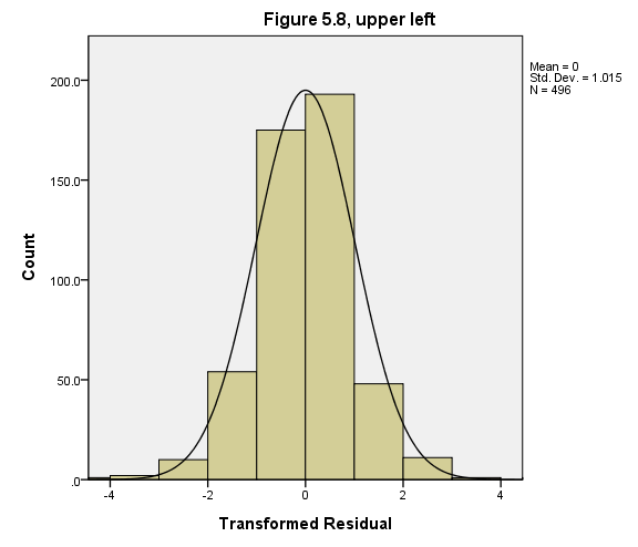
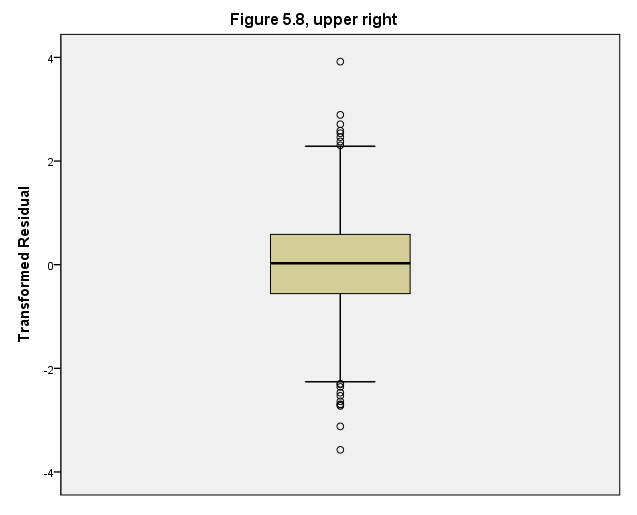
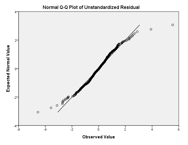
Page 157 Figure 5.8 Distribution of residuals from transformed-variables regression (Table 5.2).

GGRAPH
  /GRAPHDATASET NAME="GraphDataset" VARIABLES= resid2
  /GRAPHSPEC SOURCE=INLINE .
BEGIN GPL
SOURCE: s=userSource( id( "GraphDataset" ) )
DATA: Y_Var=col( source(s), name( "$count" ) )
DATA: resid2=col( source(s), name( "resid2" ) )
GUIDE: text.title( label( "Figure 5.8, upper left" ) )
GUIDE: axis( dim( 1 ), label( "Transformed Residual" ), delta(2) )
GUIDE: axis( dim( 2 ), label( "Count" ) )
SCALE: linear( dim( 1 ), min(-4), max(4) )
ELEMENT: interval( position( summary.count( bin.rect( resid2, binCount( 12 ) ) ) ) )
ELEMENT: line( position( density.normal( resid2 ) ) )
END GPL.

GGRAPH 
  /GRAPHDATASET NAME="graphdataset" VARIABLES=resid2 
  /GRAPHSPEC SOURCE=INLINE. 
BEGIN GPL 
SOURCE: s=userSource(id("graphdataset")) 
DATA: resid2=col(source(s), name("resid2")) 
GUIDE: text.title( label( "Figure 5.8, upper right" ))
COORD: rect(dim(1), transpose()) 
GUIDE: axis(dim(1), label("Transformed Residual"), delta(2)) 
SCALE: linear( dim( 1 ), min(-4), max(4) )
ELEMENT: schema(position(bin.quantile.letter(resid2))) 
END GPL.

NOTE: The symmetry plot has been skipped for now.

pplot
/variable = resid2
/type q-q.

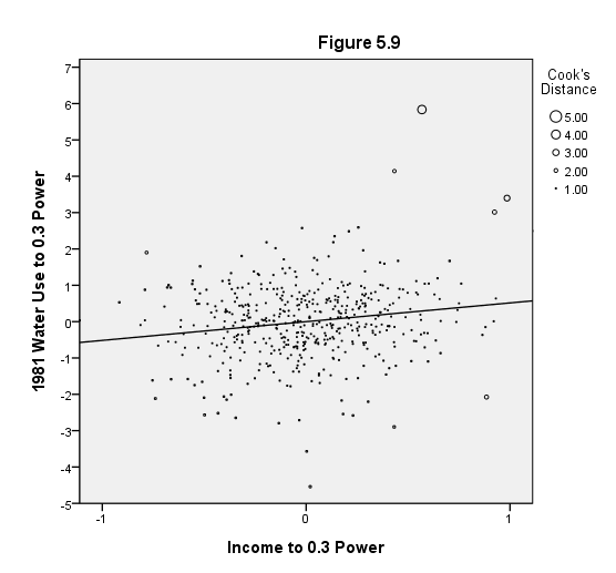
Page 157 Figure 5.9 Proportional leverage plot for transformed-variables regression: 1981 water use versus income.

REGRESSION
  /DEPENDENT y
  /METHOD=ENTER x2 educat retire x5 x7
  /SAVE RESID (resid3).

**Variables Entered/Removed(b)**
Model	Variables Entered	Variables Removed	Method
1	X7, X2, Education in Years, head of house retired?, X5(a)	.	Enter
a All requested variables entered.
b Dependent Variable: Y

**Model Summary(b)**
Model	R	R Square	Adjusted R Square	Std. Error of the Estimate
1	.843(a)	.711	.708	1.03619
a Predictors: (Constant), X7, X2, Education in Years, head of house retired?, X5
b Dependent Variable: Y

**ANOVA(b)**
Model		Sum of Squares	df	Mean Square	F	Sig.
1	Regression	1293.645	5	258.729	240.971	.000(a)
	Residual	526.109	490	1.074
	Total	1819.754	495
a Predictors: (Constant), X7, X2, Education in Years, head of house retired?, X5
b Dependent Variable: Y

**Coefficients(a)**
		Unstandardized Coefficients		Standardized Coefficients	t	Sig.
Model		B	Std. Error	Beta	t	Sig.
1	(Constant)	2.590	.343		7.553	.000
	X2	.648	.029	.679	22.348	.000
	Education in Years	-1.515E-02	.015	-.024	-.987	.324
	head of house retired?	-3.688E-02	.116	-.009	-.319	.750
	X5	.779	.111	.227	7.027	.000
	X7	.949	.267	.090	3.562	.000
a Dependent Variable: Y

**Casewise Diagnostics(a)**
Case Number	Std. Residual	Y
80	3.997	14.42
85	5.632	13.93
105	-3.446	3.98
118	3.280	14.77
125	3.203	15.46
175	-4.382	3.98
a Dependent Variable: Y

**Residuals Statistics(a)**
	Minimum	Maximum	Mean	Std. Deviation	N
Predicted Value	5.5148	14.5674	9.7770	1.61661	496
Residual	-4.5408	5.8354	.0000	1.03094	496
Std. Predicted Value	-2.636	2.963	.000	1.000	496
Std. Residual	-4.382	5.632	.000	.995	496
a Dependent Variable: Y


REGRESSION
  /DEPENDENT x1
  /METHOD=ENTER x2 educat retire x5 x7
  /SAVE RESID (resid4).

**Variables Entered/Removed(b)**
Model	Variables Entered	Variables Removed	Method
1	X7, X2, Education in Years, head of house retired?, X5(a)	.	Enter
a All requested variables entered.
b Dependent Variable: X1

**Model Summary(b)**
Model	R	R Square	Adjusted R Square	Std. Error of the Estimate
1	.612(a)	.374	.368	.35552
a Predictors: (Constant), X7, X2, Education in Years, head of house retired?, X5
b Dependent Variable: X1

**ANOVA(b)**
Model		Sum of Squares	df	Mean Square	F	Sig.
1	Regression	37.023	5	7.405	58.583	.000(a)
	Residual	61.933	490	.126
	Total	98.956	495
a Predictors: (Constant), X7, X2, Education in Years, head of house retired?, X5
b Dependent Variable: X1

**Coefficients(a)**
		Unstandardized Coefficients		Standardized Coefficients	t	Sig.
Model		B	Std. Error	Beta	t	Sig.
1	(Constant)	1.422	.118		12.092	.000
	X2	4.277E-02	.010	.192	4.302	.000
	Education in Years	4.070E-02	.005	.281	7.731	.000
	head of house retired?	-.268	.040	-.274	-6.766	.000
	X5	.125	.038	.157	3.297	.001
	X7	6.522E-02	.091	.027	.713	.476
a Dependent Variable: X1

**Casewise Diagnostics(a)**
Case Number	Std. Residual	X1
65	3.360	3.61
125	3.318	3.98
140	3.168	3.42
244	-3.124	1.62
a Dependent Variable: X1

**Residuals Statistics(a)**
	Minimum	Maximum	Mean	Std. Deviation	N
Predicted Value	1.7908	3.1666	2.4750	.27348	496
Residual	-1.1107	1.1945	.0000	.35372	496
Std. Predicted Value	-2.502	2.529	.000	1.000	496
Std. Residual	-3.124	3.360	.000	.995	496
a Dependent Variable: X1

regression
/dependent = resid3
/method = enter resid4
/save cook (cook3).

compute cook4 = $sysmis.
if cook3 <=1 cook4 = (99/4) * cook3 * (cook3 + 1) ** 2+ 1.
if cook3 > 1 cook4 = 100.
exe.

formats resid3 (f2.0) resid4 (f1.0) cook4 (f4.2).
GGRAPH
  /GRAPHDATASET NAME="graphdataset" VARIABLES=resid3 resid4 cook4
  /GRAPHSPEC SOURCE=INLINE.
BEGIN GPL
SOURCE: s=userSource(id("graphdataset"))
DATA: resid3=col(source(s), name("resid3"))
DATA: resid4=col(source(s), name("resid4"))
DATA: cook4=col(source(s), name("cook4"))
GUIDE: text.title( label( "Figure 5.9" ) )
GUIDE: axis(dim(1), delta(1), label("Income to 0.3 Power"))
GUIDE: axis(dim(2), delta(1), label("1981 Water Use to 0.3 Power"))
GUIDE: legend(aesthetic(aesthetic.size), label("Cook's Distance"))
SCALE: linear(dim(1), min(-1), max(1))
SCALE: linear(dim(2), min(-5), max(6))
ELEMENT: point(position(resid4*resid3), size(cook4))
ELEMENT: line(position(smooth.linear(resid4*resid3)))
END GPL.

Image rwgch5_9

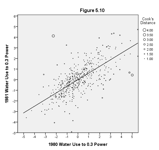
Page 158 Figure 5.10 Proportional leverage plot for transformed-variables regression: 1981 water use versus 1980 water use.

REGRESSION
   /DEPENDENT y
  /METHOD=ENTER x1 retire educat x5 x7
  /SAVE RESID (resid5).

**Variables Entered/Removed(b)**
Model	Variables Entered	Variables Removed	Method
1	X7, Education in Years, head of house retired?, X5, X1(a)	.	Enter
a All requested variables entered.
b Dependent Variable: Y

**Model Summary(b)**
Model	R	R Square	Adjusted R Square	Std. Error of the Estimate
1	.675(a)	.455	.449	1.42266
a Predictors: (Constant), X7, Education in Years, head of house retired?, X5, X1
b Dependent Variable: Y

**ANOVA(b)**
Model		Sum of Squares	df	Mean Square	F	Sig.
1	Regression	828.012	5	165.602	81.821	.000(a)
	Residual	991.741	490	2.024
	Total	1819.754	495
a Predictors: (Constant), X7, Education in Years, head of house retired?, X5, X1
b Dependent Variable: Y

**Coefficients(a)**
		Unstandardized Coefficients		Standardized Coefficients	t	Sig.
Model		B	Std. Error	Beta	t	Sig.
1	(Constant)	5.949	.466		12.759	.000
	X1	1.048	.177	.244	5.906	.000
	head of house retired?	-6.735E-02	.165	-.016	-.407	.684
	Education in Years	-3.879E-02	.022	-.063	-1.739	.083
	X5	1.843	.136	.537	13.601	.000
	X7	-5.346E-03	.361	-.001	-.015	.988
a Dependent Variable: Y

**Casewise Diagnostics(a)**
Case Number	Std. Residual	Y
69	-3.993	3.98
124	3.035	15.90
147	3.321	11.76
175	-3.458	3.98
321	3.071	11.15
a Dependent Variable: Y

**Residuals Statistics(a)**
	Minimum	Maximum	Mean	Std. Deviation	N
Predicted Value	6.7453	12.4798	9.7770	1.29335	496
Residual	-5.6800	4.7243	.0000	1.41546	496
Std. Predicted Value	-2.344	2.090	.000	1.000	496
Std. Residual	-3.993	3.321	.000	.995	496
a Dependent Variable: Y

REGRESSION
  /DEPENDENT x2
  /METHOD=ENTER x1 retire educat x5 x7
  /SAVE RESID (resid6).

**Variables Entered/Removed(b)**
Model	Variables Entered	Variables Removed	Method
1	X7, Education in Years, head of house retired?, X5, X1(a)	.	Enter
a All requested variables entered.
b Dependent Variable: X2

**Model Summary(b)**
Model	R	R Square	Adjusted R Square	Std. Error of the Estimate
1	.620(a)	.384	.378	1.58578
a Predictors: (Constant), X7, Education in Years, head of house retired?, X5, X1
b Dependent Variable: X2

**ANOVA(b)**
Model		Sum of Squares	df	Mean Square	F	Sig.
1	Regression	768.524	5	153.705	61.122	.000(a)
	Residual	1232.207	490	2.515
	Total	2000.731	495
a Predictors: (Constant), X7, Education in Years, head of house retired?, X5, X1
b Dependent Variable: X2

**Coefficients(a)**
		Unstandardized Coefficients		Standardized Coefficients	t	Sig.
Model		B	Std. Error	Beta	t	Sig.
1	(Constant)	6.543	.520		12.590	.000
	X1	.851	.198	.189	4.302	.000
	head of house retired?	-.270	.184	-.061	-1.463	.144
	Education in Years	-4.251E-03	.025	-.007	-.171	.864
	X5	1.804	.151	.501	11.942	.000
	X7	-1.472	.403	-.134	-3.657	.000
a Dependent Variable: X2

**Casewise Diagnostics(a)**
Case Number	Std. Residual	X2
56	-3.001	4.90
69	-3.175	4.90
94	3.153	17.03
147	3.473	13.10
155	3.045	14.48
362	3.479	14.71
477	3.040	14.65
a Dependent Variable: X2

**Residuals Statistics(a)**
	Minimum	Maximum	Mean	Std. Deviation	N
Predicted Value	7.2745	12.8808	10.2970	1.24602	496
Residual	-5.0356	5.5166	.0000	1.57775	496
Std. Predicted Value	-2.426	2.074	.000	1.000	496
Std. Residual	-3.175	3.479	.000	.995	496
a Dependent Variable: X2

regression
/dependent = resid5
/method = enter resid6
/save cook (cook5).

compute cook6 = $sysmis.
if cook5 <=1 cook6 = ((99/4) * cook5 * (cook5 + 1) ** 2)+ 1.
if cook5 > 1 cook6 = 100.
exe.

formats resid6 (f2.0) resid5 (f1.0) cook6 (f4.2).
 GGRAPH
  /GRAPHDATASET NAME="graphdataset" VARIABLES=resid6 resid5 cook6
  /GRAPHSPEC SOURCE=INLINE.
BEGIN GPL
SOURCE: s=userSource(id("graphdataset"))
DATA: resid6=col(source(s), name("resid6"))
DATA: resid5=col(source(s), name("resid5"))
DATA: cook6=col(source(s), name("cook6"))
GUIDE: text.title( label( "Figure 5.10" ) )
GUIDE: axis(dim(1), delta(1), label("1980 Water Use to 0.3 Power"))
GUIDE: axis(dim(2), delta(1), label("1981 Water Use to 0.3 Power"))
GUIDE: legend(aesthetic(aesthetic.size), label("Cook's Distance"))
SCALE: linear(dim(1), min(-5), max(5))
SCALE: linear(dim(2), min(-5), max(5))
ELEMENT: point(position(resid6*resid5), size(cook6))
ELEMENT: line(position(smooth.linear(resid6*resid5)))
END GPL.

Image rwgch5_10

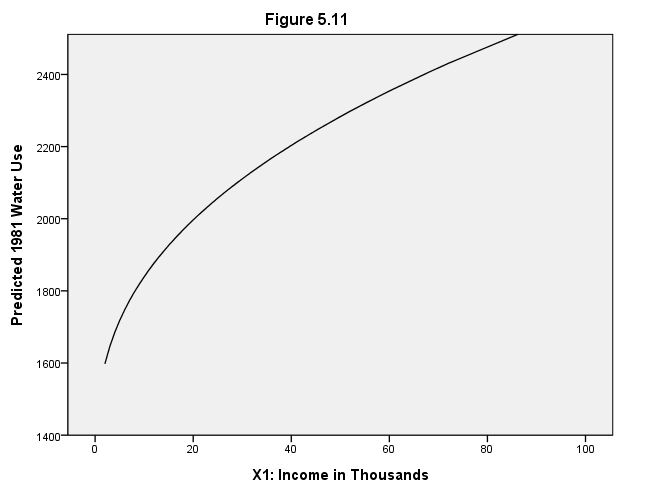
Page 160 Figure 5.11 Conditional effect plot showing curvilinear relation between 1981 water use and income, with other X variables at means.

compute yhat1=8.507+.516*(x1).
compute yhata=yhat1**(1/.3).
execute.

formats yhata (f4.0).
GGRAPH
  /GRAPHDATASET NAME="graphdataset" VARIABLES=income yhata
  /GRAPHSPEC SOURCE=INLINE.
BEGIN GPL
SOURCE: s=userSource(id("graphdataset"))
DATA: income=col(source(s), name("income"))
DATA: yhata=col(source(s), name("yhata"))
GUIDE: text.title( label( "Figure 5.11" ) )
GUIDE: axis(dim(1), delta(20), label("X1: Income in Thousands"))
GUIDE: axis(dim(2), delta(200), label("Predicted 1981 Water Use"))
SCALE: linear(dim(1), min(0), max(100))
SCALE: linear(dim(2), min(1400), max(2400))
ELEMENT: line(position(income*yhata))
END GPL.

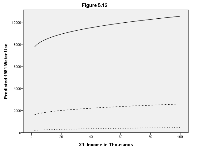
Page 161 Figure 5.12 Conditional effect plot with three levels of other X variables.

compute yhat2=14.046+.516*(x1).
compute yhatb=yhat2**(1/.3).
compute yhat1=8.507+.516*(x1).
compute yhata=yhat1**(1/.3).
compute yhat3=4.204+.516*(x1).
compute yhatc=yhat3**(1/.3).
execute.

formats yhatb yhatc (f4.0).
GGRAPH
  /GRAPHDATASET NAME="graphdataset" VARIABLES=income yhata yhatb yhatc
  /GRAPHSPEC SOURCE=INLINE.
BEGIN GPL
SOURCE: s=userSource(id("graphdataset"))
DATA: income=col(source(s), name("income"))
DATA: yhata=col(source(s), name("yhata"))
DATA: yhatb=col(source(s), name("yhatb"))
DATA: yhatc=col(source(s), name("yhatc"))
GUIDE: text.title( label( "Figure 5.12" ) )
GUIDE: axis(dim(1), delta(20), label("X1: Income in Thousands"))
GUIDE: axis(dim(2), delta(2000), label("Predicted 1981 Water Use"))
SCALE: linear(dim(1), min(0), max(100))
SCALE: linear(dim(2), min(0), max(10000))
ELEMENT: line(position(income*yhata), shape(shape.dash))
ELEMENT: line(position(income*yhatb))
ELEMENT: line(position(income*yhatc), shape(shape.half_dash))
END GPL.

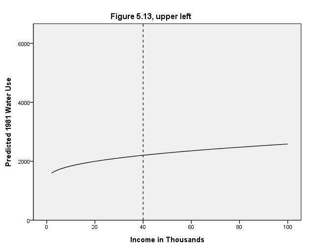
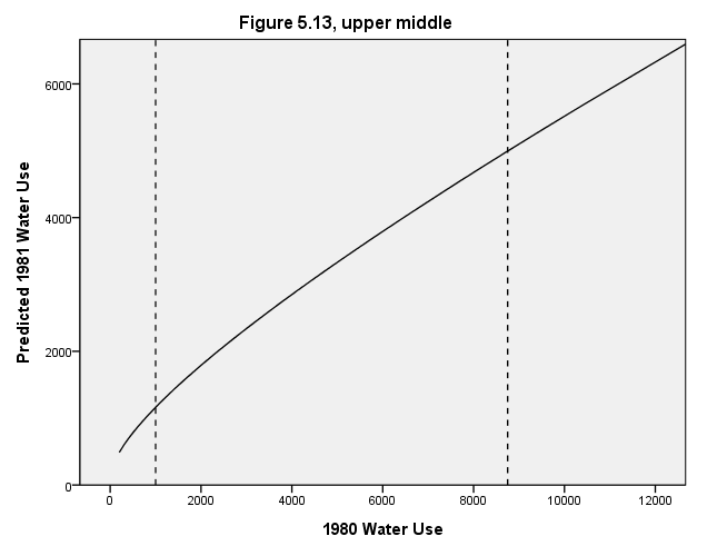
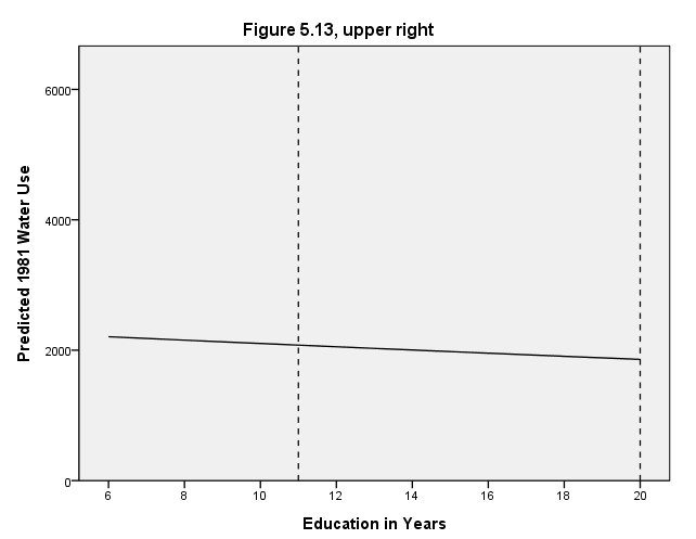
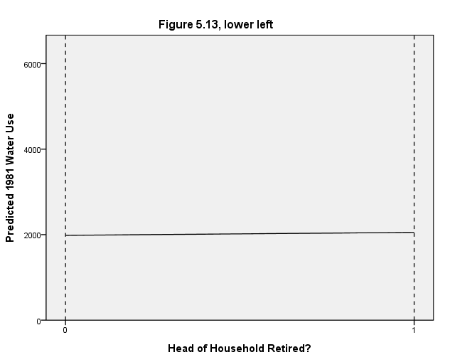
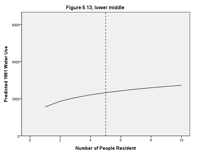
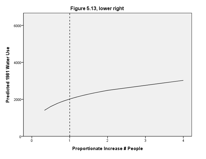
Page 162 Figure 5.13 Conditional effect plots for X variables of Equation [5.13], each with other X variables at their means.

NOTE: Some of the graphs do not look exactly as they do in the book because the y-axis is scaled differently.

Upper left graph

compute yhat1=8.507+.516*(income**.3).
compute yhata=yhat1**(1/.3).
execute.

formats yhat5131a (f4.0).
GGRAPH
  /GRAPHDATASET NAME="graphdataset" VARIABLES=income yhat5131a
  /GRAPHSPEC SOURCE=INLINE.
BEGIN GPL
SOURCE: s=userSource(id("graphdataset"))
DATA: income=col(source(s), name("income"))
DATA: yhat5131a=col(source(s), name("yhat5131a"))
GUIDE: form.line(position(40), shape(shape.dash))
GUIDE: text.title( label( "Figure 5.13, upper left" ) )
GUIDE: axis(dim(1), delta(20), label("Income in Thousands"))
GUIDE: axis(dim(2), delta(2000), label("Predicted 1981 Water Use"))
SCALE: linear(dim(1), min(0), max(100))
SCALE: linear(dim(2), min(0), max(6000))
ELEMENT: line(position(income*yhat5131a))
END GPL.

Upper middle graph

compute yhat2=3.338+.626*(water80**.3).
compute yhatb=yhat2**(1/.3).
execute.

formats yhat5132b (f4.0).
GGRAPH
  /GRAPHDATASET NAME="graphdataset" VARIABLES=water80 yhat5132b
  /GRAPHSPEC SOURCE=INLINE.
BEGIN GPL
SOURCE: s=userSource(id("graphdataset"))
DATA: water80=col(source(s), name("water80"))
DATA: yhat5132b=col(source(s), name("yhat5132b"))
GUIDE: form.line(position(1000), shape(shape.dash))
GUIDE: form.line(position(8750), shape(shape.dash))
GUIDE: text.title( label( "Figure 5.13, upper middle" ) )
GUIDE: axis(dim(1), delta(2000), label("1980 Water Use"))
GUIDE: axis(dim(2), delta(2000), label("Predicted 1981 Water Use"))
SCALE: linear(dim(1), min(0), max(12000))
SCALE: linear(dim(2), min(0), max(6000))
ELEMENT: line(position(water80*yhat5132b))
END GPL.

Upper right graph

compute yhat3=10.288-.036*(educat).
compute yhatc=yhat3**(1/.3).
execute.

formats yhat5133c (f4.0).
GGRAPH
  /GRAPHDATASET NAME="graphdataset" VARIABLES=educat yhat5133c
  /GRAPHSPEC SOURCE=INLINE.
BEGIN GPL
SOURCE: s=userSource(id("graphdataset"))
DATA: educat=col(source(s), name("educat"))
DATA: yhat5133c=col(source(s), name("yhat5133c"))
GUIDE: form.line(position(11), shape(shape.dash))
GUIDE: form.line(position(20), shape(shape.dash))
GUIDE: text.title( label( "Figure 5.13, upper right" ) )
GUIDE: axis(dim(1), delta(2), label("Education in Years"))
GUIDE: axis(dim(2), delta(2000), label("Predicted 1981 Water Use"))
SCALE: linear(dim(1), min(6), max(20))
SCALE: linear(dim(2), min(0), max(6000))
ELEMENT: line(position(educat*yhat5133c))
END GPL.

Lower left graph

compute yhat4=9.755+.101*(retire).
compute yhatd=yhat4**(1/.3).
execute.

formats yhat5134d (f4.0).
GGRAPH
  /GRAPHDATASET NAME="graphdataset" VARIABLES=retire yhat5134d
  /GRAPHSPEC SOURCE=INLINE.
BEGIN GPL
SOURCE: s=userSource(id("graphdataset"))
DATA: retire=col(source(s), name("retire"))
DATA: yhat5134d=col(source(s), name("yhat5134d"))
GUIDE: text.title( label( "Figure 5.13, lower left" ) )
GUIDE: axis(dim(1), delta(1), label("Head of Household Retired?"))
GUIDE: axis(dim(2), delta(2000), label("Predicted 1981 Water Use"))
GUIDE: form.line(position(0), shape(shape.dash))
GUIDE: form.line(position(1), shape(shape.dash))
SCALE: linear(dim(1), min(0), max(1))
SCALE: linear(dim(2), min(0), max(6000))
ELEMENT: line(position(retire*yhat5134d))
END GPL.

Lower middle graph

compute yhat5=9.087+.715*(ln(peop81)).
compute yhate=yhat5**(1/.3).
execute.

formats yhat5135e (f4.0).
GGRAPH
  /GRAPHDATASET NAME="graphdataset" VARIABLES=peop81 yhat5135e
  /GRAPHSPEC SOURCE=INLINE.
BEGIN GPL
SOURCE: s=userSource(id("graphdataset"))
DATA: peop81=col(source(s), name("peop81"))
DATA: yhat5135e=col(source(s), name("yhat5135e"))
GUIDE: form.line(position(5), shape(shape.dash))
GUIDE: text.title( label( "Figure 5.13, lower middle" ) )
GUIDE: axis(dim(1), delta(2), label("Number of People Resident"))
GUIDE: axis(dim(2), delta(2000), label("Predicted 1981 Water Use"))
SCALE: linear(dim(1), min(0), max(10))
SCALE: linear(dim(2), min(0), max(6000))
ELEMENT: line(position(peop81*yhat5135e))
END GPL.

Lower right graph

compute x=peop81/peop80.
compute yhat6=9.802+.916*(ln(x)).
compute yhatf=yhat6**(1/.3).
execute.

formats yhat5136f (f4.0) x (f1.0).
GGRAPH
  /GRAPHDATASET NAME="graphdataset" VARIABLES=x yhat5136f
  /GRAPHSPEC SOURCE=INLINE.
BEGIN GPL
SOURCE: s=userSource(id("graphdataset"))
DATA: x=col(source(s), name("x"))
DATA: yhat5136f=col(source(s), name("yhat5136f"))
GUIDE: form.line(position(1), shape(shape.dash))
GUIDE: text.title( label( "Figure 5.13, lower right" ) )
GUIDE: axis(dim(1), delta(1), label("Proportionate Increase # People"))
GUIDE: axis(dim(2), delta(2000), label("Predicted 1981 Water Use"))
SCALE: linear(dim(1), min(0), max(4))
SCALE: linear(dim(2), min(0), max(6000))
ELEMENT: line(position(x*yhat5136f))
END GPL.

Page 168 Table 5.3 Percentage of women with at least one child, by women’s age and year of birth (England and Wales).

GET FILE 'd:appsrwgdatachild.sav'.

USE ALL.
COMPUTE filter_$=( ~  SYSMIS(c1930)).
VARIABLE LABEL filter_$ ' ~  SYSMIS(c1930)(FILTER)'.
VALUE LABELS filter_$  0 'Not Selected' 1 'Selected'.
FORMAT filter_$ (f1.0).
FILTER BY filter_$.
EXECUTE .

list age c1920 c1930 c1940 c1945 c1950 c1955 c1960.

     AGE    C1920    C1930    C1940    C1945    C1950    C1955    C1960

      15        0        0        0        0        0        0        0
      20        7        9       13       17       19       18       13
      25       39       48       59       60       53       45       39
      30       67       75       82       82       75       68        .
      35       76       83       87       88       83        .        .
      40       78       86       89       90        .        .        .
      45        .       86       89        .        .        .        .

Number of cases read:  7    Number of cases listed:  7

Page 169 Table 5.4 Iterative least squares (modified Gauss-Newton method) fitting of Gompertz curve to 1945 cohort data from Table 5.3.

MODEL PROGRAM ALPHA=89 GAMMA=942 BETA=.31 .
COMPUTE PRED_ = alpha * EXP(-gamma * EXP(-beta*age)).
NLR c1945
  /PRED PRED_
  /CRITERIA ITER 10 SSCONVERGENCE 1E-8 PCON 1E-8 .

All the derivatives will be calculated numerically.

 Iteration  Residual SS       ALPHA       GAMMA        BETA

     1      17.54197876  89.0000000  942.000000  .310000000
     1.1    598.7981763  90.3871209  237.637489  .279797958
     1.2    5.742187401  89.3300064  848.215504  .309101970
     2      5.742187401  89.3300064  848.215504  .309101970
     2.1    3.542903094  89.5395782  729.009914  .302657448
     3      3.542903094  89.5395782  729.009914  .302657448
     3.1    3.278677871  90.0387437  532.145066  .289695708
     4      3.278677871  90.0387437  532.145066  .289695708
     4.1    .1714903417  90.3584739  474.489717  .282616457
     5      .1714903417  90.3584739  474.489717  .282616457
     5.1    .1184341179  90.4253381  467.907296  .281692144

Run stopped after 11 model evaluations and 5 derivative evaluations.
The iterations limit has been reached.

Nonlinear Regression Summary Statistics     Dependent Variable C1945

  Source                 DF  Sum of Squares  Mean Square

  Regression              3    26456.88157     8818.96052
  Residual                3         .11843         .03948
  Uncorrected Total       6    26457.00000

  (Corrected Total)       5     7528.83333

  R squared = 1 - Residual SS / Corrected SS =     .99998

                                           Asymptotic 95 %
                          Asymptotic     Confidence Interval
  Parameter   Estimate    Std. Error     Lower         Upper

  ALPHA     90.425338128   .160165402 89.915620337 90.935055918
  GAMMA     467.90729568 22.934583679 394.91921459 540.89537677
  BETA        .281692144   .002228173   .274601103   .288783184

  Asymptotic Correlation Matrix of the Parameter Estimates

               ALPHA     GAMMA      BETA

  ALPHA       1.0000    -.5859    -.6330
  GAMMA       -.5859    1.0000     .9927
  BETA        -.6330     .9927    1.0000

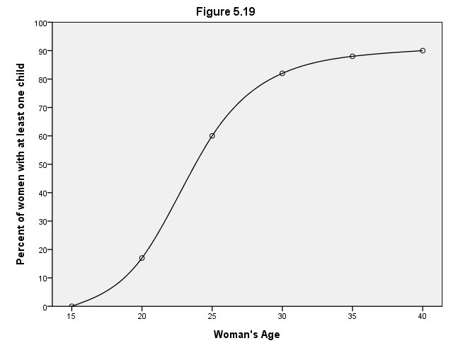
Page 169 Figure 5.19 Gompertz curve fit to 1945 cohort data from Table 5.3.

formats age (f2.0) c1945 (f2.0).
GGRAPH
  /GRAPHDATASET NAME="graphdataset" VARIABLES=age c1945
  /GRAPHSPEC SOURCE=INLINE.
BEGIN GPL
SOURCE: s=userSource(id("graphdataset"))
DATA: age=col(source(s), name("age"))
DATA: c1945=col(source(s), name("c1945"))
GUIDE: text.title( label( "Figure 5.19" ) )
GUIDE: axis(dim(1), delta(5), label("Woman's Age"))
GUIDE: axis(dim(2), delta(10), label("Percent of women with at least one child"))
SCALE: linear(dim(1), min(15), max(40))
SCALE: linear(dim(2), min(0), max(90))
ELEMENT: line(position(smooth.spline(age*c1945)))
ELEMENT: point(position(age*c1945))
END GPL.

Page 170 Table 5.5 Results from nonlinear regression fitting Gompertz curve to 1945 cohort data (Tables 5.3 and 5.4).

MODEL PROGRAM ALPHA=89 GAMMA=942 BETA=.31 .
COMPUTE PRED_ = alpha*EXP(-gamma*EXP(-beta*age)).
NLR c1945
  /PRED PRED_
  /CRITERIA SSCONVERGENCE 1E-8 PCON 1E-8.

All the derivatives will be calculated numerically.

 Iteration  Residual SS       ALPHA       GAMMA        BETA

     1      17.54197876  89.0000000  942.000000  .310000000
     1.1    598.7981763  90.3871209  237.637489  .279797958
     1.2    5.742187401  89.3300064  848.215504  .309101970
     2      5.742187401  89.3300064  848.215504  .309101970
     2.1    3.542903094  89.5395782  729.009914  .302657448
     3      3.542903094  89.5395782  729.009914  .302657448
     3.1    3.278677871  90.0387437  532.145066  .289695708
     4      3.278677871  90.0387437  532.145066  .289695708
     4.1    .1714903417  90.3584739  474.489717  .282616457
     5      .1714903417  90.3584739  474.489717  .282616457
     5.1    .1184341179  90.4253381  467.907296  .281692144
     6      .1184341179  90.4253381  467.907296  .281692144
     6.1    .1184226504  90.4253401  468.057740  .281702774
     7      .1184226504  90.4253401  468.057740  .281702774
     7.1    .1184226504  90.4253417  468.057480  .281702744

Run stopped after 15 model evaluations and 7 derivative evaluations.
Iterations have been stopped because the relative reduction between successive
residual sums of squares is at most SSCON = 1.000E-08

Nonlinear Regression Summary Statistics     Dependent Variable C1945

  Source                 DF  Sum of Squares  Mean Square

  Regression              3    26456.88158     8818.96053
  Residual                3         .11842         .03947
  Uncorrected Total       6    26457.00000

  (Corrected Total)       5     7528.83333

  R squared = 1 - Residual SS / Corrected SS =     .99998

                                           Asymptotic 95 %
                          Asymptotic     Confidence Interval
  Parameter   Estimate    Std. Error     Lower         Upper

  ALPHA     90.425341697   .160668948 89.914021396 90.936661998
  GAMMA     468.05748025 22.546420712 396.30470696 539.81025355
  BETA        .281702744   .002218428   .274642716   .288762772

  Asymptotic Correlation Matrix of the Parameter Estimates

               ALPHA     GAMMA      BETA

  ALPHA       1.0000    -.5869    -.6342
  GAMMA       -.5869    1.0000     .9927
  BETA        -.6342     .9927    1.0000

NOTE: Due to differences in the implementation of the calculations between Stata (the statistical package used by Hamilton) and SPSS, some of the values in the table (namely the sums of squares) are different. However, the important point is that the parameter estimates are the same.

Page 172 Table 5.6 Gompertz parameter estimates for fertility data (Table 5.3).

MODEL PROGRAM ALPHA=89 GAMMA=942 BETA=.31 .
COMPUTE PRED_ = alpha*EXP(-gamma*EXP(-beta*age)).
NLR c1920
  /PRED PRED_
  /CRITERIA SSCONVERGENCE 1E-8 PCON 1E-8.

Non-linear Regression

All the derivatives will be calculated numerically.

 Iteration  Residual SS       ALPHA       GAMMA        BETA

     1      908.6557474  89.0000000  942.000000  .310000000
     1.1    11986351023  79.3874151  -252.27538  .236826604
     1.2    378.4232069  85.8568703  1037.02914  .304985988
     2      378.4232069  85.8568703  1037.02914  .304985988
     2.1    10.31631948  78.2960788  1009.05972  .294390347
     3      10.31631948  78.2960788  1009.05972  .294390347
     3.1    126.4557206  79.2948835  388.987396  .266987014
     3.2    7.977538060  78.4389183  962.184891  .290877218
     4      7.977538060  78.4389183  962.184891  .290877218
     4.1    6.353976630  78.6917786  833.978224  .285130398
     5      6.353976630  78.6917786  833.978224  .285130398
     5.1    6.022247176  79.1567836  598.096516  .272939711
     6      6.022247176  79.1567836  598.096516  .272939711
     6.1    3.004750710  79.4433989  529.661441  .266133785
     7      3.004750710  79.4433989  529.661441  .266133785
     7.1    2.868076801  79.7811081  452.873041  .259685285
     8      2.868076801  79.7811081  452.873041  .259685285
     8.1    2.727895377  79.7784101  458.714108  .259774633
     9      2.727895377  79.7784101  458.714108  .259774633
     9.1    2.727543220  79.7703216  461.039073  .259978531
    10      2.727543220  79.7703216  461.039073  .259978531
    10.1    2.727541378  79.7705981  461.074794  .259979928
    11      2.727541378  79.7705981  461.074794  .259979928
    11.1    2.727541373  79.7705686  461.083543  .259980697

Run stopped after 24 model evaluations and 11 derivative evaluations.
Iterations have been stopped because the relative reduction between successive
residual sums of squares is at most SSCON = 1.000E-08

Nonlinear Regression Summary Statistics     Dependent Variable C1920

  Source                 DF  Sum of Squares  Mean Square

  Regression              3    17916.27246     5972.09082
  Residual                3        2.72754         .90918
  Uncorrected Total       6    17919.00000

  (Corrected Total)       5     6037.50000

  R squared = 1 - Residual SS / Corrected SS =     .99955

                                           Asymptotic 95 %
                          Asymptotic     Confidence Interval
  Parameter   Estimate    Std. Error     Lower         Upper

  ALPHA     79.770568575   .911955897 76.868317900 82.672819250
  GAMMA     461.08354282 129.73230562 48.217446126 873.94963951
  BETA        .259980697   .011940308   .221981308   .297980086

  Asymptotic Correlation Matrix of the Parameter Estimates

               ALPHA     GAMMA      BETA

  ALPHA       1.0000    -.6347    -.6831
  GAMMA       -.6347    1.0000     .9934
  BETA        -.6831     .9934    1.0000

MODEL PROGRAM ALPHA=89 GAMMA=942 BETA=.31 .
COMPUTE PRED_= alpha*EXP(-gamma*EXP(-beta*age)).
NLR c1930
  /PRED PRED_
  /CRITERIA SSCONVERGENCE 1E-8 PCON 1E-8.

All the derivatives will be calculated numerically.

 Iteration  Residual SS       ALPHA       GAMMA        BETA

     1      224.4977158  89.0000000  942.000000  .310000000
     1.1    1061.002669  86.3443975  172.385023  .261599698
     1.2    10.94962991  85.7813291  1028.55213  .302929647
     2      10.94962991  85.7813291  1028.55213  .302929647
     2.1    8.058888711  86.0229036  682.369609  .286367802
     3      8.058888711  86.0229036  682.369609  .286367802
     3.1    2.702314631  86.4926552  502.664523  .271922111
     4      2.702314631  86.4926552  502.664523  .271922111
     4.1    .6050474327  86.5179815  532.295902  .272721482
     5      .6050474327  86.5179815  532.295902  .272721482
     5.1    .5988238506  86.5104870  537.821211  .273081207
     6      .5988238506  86.5104870  537.821211  .273081207
     6.1    .5988167972  86.5104650  537.928453  .273086587
     7      .5988167972  86.5104650  537.928453  .273086587
     7.1    .5988167964  86.5104609  537.931483  .273086809

Run stopped after 15 model evaluations and 7 derivative evaluations.
Iterations have been stopped because the relative reduction between successive
residual sums of squares is at most SSCON = 1.000E-08

Nonlinear Regression Summary Statistics     Dependent Variable C1930

  Source                 DF  Sum of Squares  Mean Square

  Regression              3    29690.40118     9896.80039
  Residual                4         .59882         .14970
  Uncorrected Total       7    29691.00000

  (Corrected Total)       6     8295.42857

  R squared = 1 - Residual SS / Corrected SS =     .99993

                                           Asymptotic 95 %
                          Asymptotic     Confidence Interval
  Parameter   Estimate    Std. Error     Lower         Upper

  ALPHA     86.510460860   .260064846 85.788405090 87.232516630
  GAMMA     537.93148323 51.257114000 395.61891996 680.24404650
  BETA        .273086809   .004078911   .261761935   .284411682

  Asymptotic Correlation Matrix of the Parameter Estimates

               ALPHA     GAMMA      BETA

  ALPHA       1.0000    -.5119    -.5603
  GAMMA       -.5119    1.0000     .9924
  BETA        -.5603     .9924    1.0000

MODEL PROGRAM ALPHA=89 GAMMA=942 BETA=.31 .
COMPUTE PRED_ = alpha*EXP(-gamma*EXP(-beta*age)).
NLR c1940
  /PRED PRED_
  /CRITERIA SSCONVERGENCE 1E-8 PCON 1E-8.

All the derivatives will be calculated numerically.

 Iteration  Residual SS       ALPHA       GAMMA        BETA

     1      .5173660836  89.0000000  942.000000  .310000000
     1.1    .4121401809  89.1041290  941.483140  .309538712
     2      .4121401809  89.1041290  941.483140  .309538712
     2.1    .4121351967  89.1038644  941.972192  .309562122
     3      .4121351967  89.1038644  941.972192  .309562122
     3.1    .4121351966  89.1038673  941.971100  .309562056

Run stopped after 6 model evaluations and 3 derivative evaluations.
Iterations have been stopped because the relative reduction between successive
residual sums of squares is at most SSCON = 1.000E-08

Nonlinear Regression Summary Statistics     Dependent Variable C1940

  Source                 DF  Sum of Squares  Mean Square

  Regression              3    33784.58786    11261.52929
  Residual                4         .41214         .10303
  Uncorrected Total       7    33785.00000

  (Corrected Total)       6     8704.85714

  R squared = 1 - Residual SS / Corrected SS =     .99995

                                           Asymptotic 95 %
                          Asymptotic     Confidence Interval
  Parameter   Estimate    Std. Error     Lower         Upper

  ALPHA     89.103867268   .195788987 88.560269894 89.647464642
  GAMMA     941.97110043 75.353364507 732.75662038 1151.1855805
  BETA        .309562056   .003586361   .299604722   .319519391

  Asymptotic Correlation Matrix of the Parameter Estimates

               ALPHA     GAMMA      BETA

  ALPHA       1.0000    -.4639    -.5082
  GAMMA       -.4639    1.0000     .9925
  BETA        -.5082     .9925    1.0000

MODEL PROGRAM ALPHA=89 GAMMA=942 BETA=.31 .
COMPUTE PRED_ =alpha*EXP(-gamma*EXP(-beta*age)).
NLR c1945
  /PRED PRED_
  /CRITERIA SSCONVERGENCE 1E-8 PCON 1E-8.

All the derivatives will be calculated numerically.

 Iteration  Residual SS       ALPHA       GAMMA        BETA

     1      17.54197876  89.0000000  942.000000  .310000000
     1.1    598.7981763  90.3871209  237.637489  .279797958
     1.2    5.742187401  89.3300064  848.215504  .309101970
     2      5.742187401  89.3300064  848.215504  .309101970
     2.1    3.542903094  89.5395782  729.009914  .302657448
     3      3.542903094  89.5395782  729.009914  .302657448
     3.1    3.278677871  90.0387437  532.145066  .289695708
     4      3.278677871  90.0387437  532.145066  .289695708
     4.1    .1714903417  90.3584739  474.489717  .282616457
     5      .1714903417  90.3584739  474.489717  .282616457
     5.1    .1184341179  90.4253381  467.907296  .281692144
     6      .1184341179  90.4253381  467.907296  .281692144
     6.1    .1184226504  90.4253401  468.057740  .281702774
     7      .1184226504  90.4253401  468.057740  .281702774
     7.1    .1184226504  90.4253417  468.057480  .281702744

Run stopped after 15 model evaluations and 7 derivative evaluations.
Iterations have been stopped because the relative reduction between successive
residual sums of squares is at most SSCON = 1.000E-08

Nonlinear Regression Summary Statistics     Dependent Variable C1945

  Source                 DF  Sum of Squares  Mean Square

  Regression              3    26456.88158     8818.96053
  Residual                3         .11842         .03947
  Uncorrected Total       6    26457.00000

  (Corrected Total)       5     7528.83333

  R squared = 1 - Residual SS / Corrected SS =     .99998

                                           Asymptotic 95 %
                          Asymptotic     Confidence Interval
  Parameter   Estimate    Std. Error     Lower         Upper

  ALPHA     90.425341697   .160668948 89.914021396 90.936661998
  GAMMA     468.05748025 22.546420712 396.30470696 539.81025355
  BETA        .281702744   .002218428   .274642716   .288762772

  Asymptotic Correlation Matrix of the Parameter Estimates

               ALPHA     GAMMA      BETA

  ALPHA       1.0000    -.5869    -.6342
  GAMMA       -.5869    1.0000     .9927
  BETA        -.6342     .9927    1.0000

MODEL PROGRAM ALPHA=89 GAMMA=942 BETA=.31 .
COMPUTE PRED_ = alpha*EXP(-gamma*EXP(-beta*age)).
NLR c1950
  /PRED PRED_
  /CRITERIA SSCONVERGENCE 1E-8 PCON 1E-8.

All the derivatives will be calculated numerically.

 Iteration  Residual SS       ALPHA       GAMMA        BETA

     1      137.5930268  89.0000000  942.000000  .310000000
     1.1     8.2171E+31  86.3356573  -921.53948  .223429666
     1.2    41.57904419  82.9023054  831.758140  .308048672
     2      41.57904419  82.9023054  831.758140  .308048672
     2.1    40.77877227  82.5582685  475.895093  .290058760
     3      40.77877227  82.5582685  475.895093  .290058760
     3.1    17.08147484  82.9509077  416.843828  .278697446
     4      17.08147484  82.9509077  416.843828  .278697446
     4.1    18.98979815  84.4091222  260.188231  .259860366
     4.2    12.52525495  83.7507578  352.608016  .270411582
     5      12.52525495  83.7507578  352.608016  .270411582
     5.1    11.00940628  84.8769170  240.482884  .254588020
     6      11.00940628  84.8769170  240.482884  .254588020
     6.1    3.245426694  85.6048322  211.953637  .245864035
     7      3.245426694  85.6048322  211.953637  .245864035
     7.1    5.830978718  86.9758776  148.690831  .231143834
     7.2    2.231916705  86.1094568  194.275142  .241405243
     8      2.231916705  86.1094568  194.275142  .241405243
     8.1    1.516254268  86.8854122  160.517741  .232915190
     9      1.516254268  86.8854122  160.517741  .232915190
     9.1    .9186875211  87.5146650  142.929543  .226819932
    10      .9186875211  87.5146650  142.929543  .226819932
    10.1    .8549764665  87.5084675  145.064663  .227214201
    11      .8549764665  87.5084675  145.064663  .227214201
    11.1    .8549348950  87.5147899  144.878812  .227148676
    12      .8549348950  87.5147899  144.878812  .227148676
    12.1    .8549348093  87.5144797  144.889648  .227152113
    13      .8549348093  87.5144797  144.889648  .227152113
    13.1    .8549348090  87.5145012  144.888925  .227151880

Run stopped after 29 model evaluations and 13 derivative evaluations.
Iterations have been stopped because the relative reduction between successive
residual sums of squares is at most SSCON = 1.000E-08

Nonlinear Regression Summary Statistics     Dependent Variable C1950

  Source                 DF  Sum of Squares  Mean Square

  Regression              3    15683.14507     5227.71502
  Residual                2         .85493         .42747
  Uncorrected Total       5    15684.00000

  (Corrected Total)       4     5104.00000

  R squared = 1 - Residual SS / Corrected SS =     .99983

                                           Asymptotic 95 %
                          Asymptotic     Confidence Interval
  Parameter   Estimate    Std. Error     Lower         Upper

  ALPHA     87.514501164  1.021149501 83.120849475 91.908152853
  GAMMA     144.88892548 24.277151687 40.432772501 249.34507845
  BETA        .227151880   .008014086   .192670052   .261633708

  Asymptotic Correlation Matrix of the Parameter Estimates

               ALPHA     GAMMA      BETA

  ALPHA       1.0000    -.7742    -.8224
  GAMMA       -.7742    1.0000     .9927
  BETA        -.8224     .9927    1.0000

MODEL PROGRAM ALPHA=89 GAMMA=942 BETA=.31 .
COMPUTE PRED_ = alpha*EXP(-gamma*EXP(-beta*age)).
NLR c1955
  /PRED PRED_
  /CRITERIA SSCONVERGENCE 1E-8 PCON 1E-8.

All the derivatives will be calculated numerically.

 Iteration  Residual SS       ALPHA       GAMMA        BETA

     1      414.8892555  89.0000000  942.000000  .310000000
     1.1     6.0073E+97  82.0855371  -1675.9821  .182700339
     1.2    77.60551524  76.0761033  887.460743  .307497672
     2      77.60551524  76.0761033  887.460743  .307497672
     2.1    202.4827259  72.2923632  284.323546  .281986292
     2.2    50.73748249  71.9647707  805.615241  .307559869
     3      50.73748249  71.9647707  805.615241  .307559869
     3.1    40.35892336  70.7386920  581.111129  .297846958
     4      40.35892336  70.7386920  581.111129  .297846958
     4.1    46.47097326  72.1282057  320.894581  .274314566
     4.2    35.15800201  71.0177581  496.223111  .289325331
     5      35.15800201  71.0177581  496.223111  .289325331
     5.1    29.92550222  72.3180935  357.359288  .274583135
     6      29.92550222  72.3180935  357.359288  .274583135
     6.1    73.55788880  75.0800949  164.833364  .245173034
     6.2    25.94374252  72.8276767  339.629252  .269775849
     7      25.94374252  72.8276767  339.629252  .269775849
     7.1    22.72862955  73.7819205  291.075788  .262132073
     8      22.72862955  73.7819205  291.075788  .262132073
     8.1    19.35346093  75.4453338  207.262951  .247057254
     9      19.35346093  75.4453338  207.262951  .247057254
     9.1    13.31842255  77.4272022  154.127080  .231500962
    10      13.31842255  77.4272022  154.127080  .231500962
    10.1    76.00147779  81.9191445  72.8384780  .202402143
    10.2    10.67467401  78.2455791  149.508531  .227849301
    11      10.67467401  78.2455791  149.508531  .227849301
    11.1    9.098115395  79.3739689  132.692956  .221822234
    12      9.098115395  79.3739689  132.692956  .221822234
    12.1    7.533534505  81.3675322  103.287965  .210112687
    13      7.533534505  81.3675322  103.287965  .210112687
    13.1    5.250820645  83.7232482  83.2478120  .198519028
    14      5.250820645  83.7232482  83.2478120  .198519028
    14.1    20.84611947  88.6976047  51.5339972  .177357084
    14.2    4.372772912  84.5625662  81.2398048  .196019014
    15      4.372772912  84.5625662  81.2398048  .196019014
    15.1    3.979864529  85.6570577  74.6683826  .191698995
    16      3.979864529  85.6570577  74.6683826  .191698995
    16.1    3.854560789  87.8080885  62.9235585  .183225072
    17      3.854560789  87.8080885  62.9235585  .183225072
    17.1    3.490601546  88.8530634  60.3798552  .180218225
    18      3.490601546  88.8530634  60.3798552  .180218225
    18.1    3.489426172  88.9373656  60.3323811  .180108558
    19      3.489426172  88.9373656  60.3323811  .180108558
    19.1    3.489422845  88.9480760  60.2920633  .180072909
    20      3.489422845  88.9480760  60.2920633  .180072909
    20.1    3.489422726  88.9465621  60.2993069  .180078937
    21      3.489422726  88.9465621  60.2993069  .180078937
    21.1    3.489422721  88.9469035  60.2977372  .180077617

Run stopped after 48 model evaluations and 21 derivative evaluations.
Iterations have been stopped because the relative reduction between successive
residual sums of squares is at most SSCON = 1.000E-08

Nonlinear Regression Summary Statistics     Dependent Variable C1955

  Source                 DF  Sum of Squares  Mean Square

  Regression              3     6969.51058     2323.17019
  Residual                1        3.48942        3.48942
  Uncorrected Total       4     6973.00000

  (Corrected Total)       3     2682.75000

  R squared = 1 - Residual SS / Corrected SS =     .99870

                                           Asymptotic 95 %
                          Asymptotic     Confidence Interval
  Parameter   Estimate    Std. Error     Lower         Upper

  ALPHA     88.946903488 10.493055191 -44.38000407 222.27381105
  GAMMA     60.297737236 37.915981908 -421.4704917 542.06596613
  BETA        .180077617   .033323126  -.243332842   .603488076

  Asymptotic Correlation Matrix of the Parameter Estimates

               ALPHA     GAMMA      BETA

  ALPHA       1.0000    -.9078    -.9442
  GAMMA       -.9078    1.0000     .9937
  BETA        -.9442     .9937    1.0000

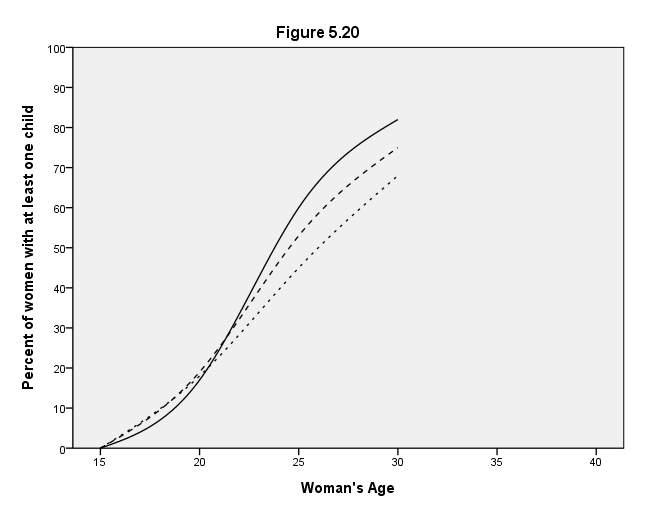
Page 172 Figure 5.20 Gompertz curves for 1945, 1950, and 1955 cohort data (see Table 5.6).

formats c1945 c1950 c1955 (f2.0).
GGRAPH
  /GRAPHDATASET NAME="graphdataset" VARIABLES=age c1945 c1950 c1955
  /GRAPHSPEC SOURCE=INLINE.
BEGIN GPL
SOURCE: s=userSource(id("graphdataset"))
DATA: age=col(source(s), name("age"))
DATA: c1945=col(source(s), name("c1945"))
DATA: c1950=col(source(s), name("c1950"))
DATA: c1955=col(source(s), name("c1955"))
GUIDE: text.title( label( "Figure 5.20" ) )
GUIDE: axis(dim(1), delta(5), label("Woman's Age"))
GUIDE: axis(dim(2), delta(10), label("Percent of women with at least one child"))
SCALE: linear(dim(1), min(15), max(40))
SCALE: linear(dim(2), min(0), max(90))
ELEMENT: line(position(smooth.spline(age*c1945))) 
ELEMENT: line(position(smooth.spline(age*c1950)), shape(shape.dash))
ELEMENT: line(position(smooth.spline(age*c1955)), shape(shape.half_dash))
END GPL.