Limitations of linear regression
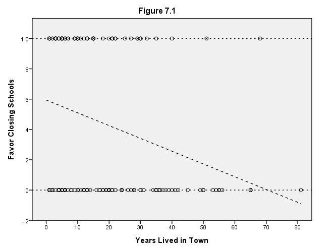
Page 218 Figure 7.1 Linear regression of a dichotomous Y variable (0 = open schools, 1 = close schools) on a measurement X variable (years lived in town).
GET FILE 'd:appsrwgdatatoxic.sav'.

formats lived (f2.0) close (f2.1).
GGRAPH
  /GRAPHDATASET NAME="graphdataset" VARIABLES=lived close
  /GRAPHSPEC SOURCE=INLINE.
BEGIN GPL
SOURCE: s=userSource(id("graphdataset"))
DATA: lived=col(source(s), name("lived"))
DATA: close=col(source(s), name("close"))
GUIDE: text.title( label( "Figure 7.1" ) )
GUIDE: form.line(position(*, 1), shape(shape.half_dash))
GUIDE: form.line(position(*, 0), shape(shape.half_dash))
GUIDE: axis(dim(1), label("Years Lived in Town"), delta(10))
GUIDE: axis(dim(2), label("Favor Closing Schools"), delta(.2))
SCALE: linear(dim(1), min(0), max(80))
SCALE: linear(dim(2), min(-.2), max(1))
ELEMENT: point(position(lived*close))
ELEMENT: line(position(smooth.linear(lived*close)), shape(shape.dash))
END GPL.
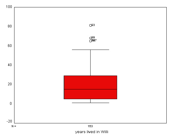
Page 219 Figure 7.2 Boxplots and oneway scatterplots of years lived in town, for respondents favoring closed and open schools.
compute const=.01.
execute.

EXAMINE  VARIABLES=lived BY close
 /PLOT=BOXPLOT
 /STATISTICS=NONE.
| |
Cases | |||||
|---|---|---|---|---|---|---|
| Valid | Missing | Total | ||||
| N | Percent | N | Percent | N | Percent | |
| years lived in Williamstown | 153 | 100.0% | 0 | .0% | 153 | 100.0% |
| |
Cases | ||||||
|---|---|---|---|---|---|---|---|
| Valid | Missing | Total | |||||
| schools should close | N | Percent | N | Percent | N | Percent | |
| years lived in Williamstown | open | 87 | 100.0% | 0 | .0% | 87 | 100.0% |
| close | 66 | 100.0% | 0 | .0% | 66 | 100.0% | |
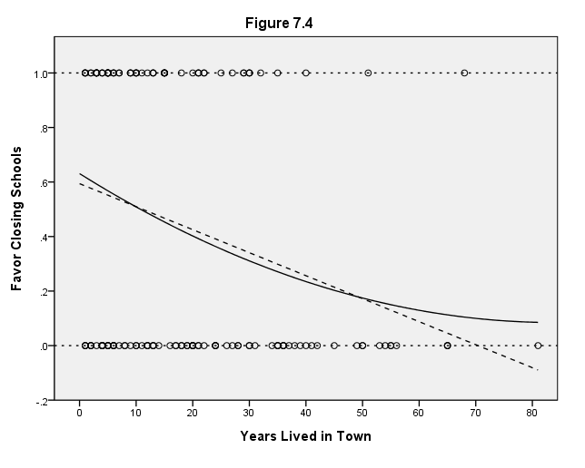
Page 222 Figure 7.4 Logit regression of school-closing opinion on years lived in town, also showing linear regression line.
GGRAPH
  /GRAPHDATASET NAME="graphdataset" VARIABLES=lived close
  /GRAPHSPEC SOURCE=INLINE.
BEGIN GPL
SOURCE: s=userSource(id("graphdataset"))
DATA: lived=col(source(s), name("lived"))
DATA: close=col(source(s), name("close"))
GUIDE: text.title( label( "Figure 7.4" ) )
GUIDE: form.line(position(*, 1), shape(shape.half_dash))
GUIDE: form.line(position(*, 0), shape(shape.half_dash))
GUIDE: axis(dim(1), label("Years Lived in Town"), delta(10))
GUIDE: axis(dim(2), label("Favor Closing Schools"), delta(.2))
SCALE: linear(dim(1), min(0), max(80))
SCALE: linear(dim(2), min(-.2), max(1))
ELEMENT: point(position(lived*close))
ELEMENT: line(position(smooth.linear(lived*close)), shape(shape.dash))
ELEMENT: line(position(smooth.quadratic(lived*close)))
END GPL.
Page 224 Table 7.1 Logit regression of school-closing opinion on years lived in town.
LOGISTIC REGRESSION VAR=close
  /METHOD=ENTER lived.
| Unweighted Cases(a) | N | Percent | |
|---|---|---|---|
| Selected Cases | Included in Analysis | 153 | 100.0 |
| Missing Cases | 0 | .0 | |
| Total | 153 | 100.0 | |
| Unselected Cases | 0 | .0 | |
| Total | 153 | 100.0 | |
| a If weight is in effect, see classification table for the total number of cases. | |||
| Original Value | Internal Value |
|---|---|
| open | 0 |
| close | 1 |
| |
Predicted | ||||
|---|---|---|---|---|---|
| schools should close | Percentage Correct | ||||
| Observed | open | close | |||
| Step 0 | schools should close | open | 87 | 0 | 100.0 |
| close | 66 | 0 | .0 | ||
| Overall Percentage | |
|
56.9 | ||
| a Constant is included in the model. | |||||
| b The cut value is .500 | |||||
| |
B | S.E. | Wald | df | Sig. | Exp(B) | |
|---|---|---|---|---|---|---|---|
| Step 0 | Constant | -.276 | .163 | 2.864 | 1 | .091 | .759 |
| |
Score | df | Sig. | ||
|---|---|---|---|---|---|
| Step 0 | Variables | LIVED | 12.683 | 1 | .000 |
| Overall Statistics | 12.683 | 1 | .000 | ||
| |
Chi-square | df | Sig. | |
|---|---|---|---|---|
| Step 1 | Step | 13.944 | 1 | .000 |
| Block | 13.944 | 1 | .000 | |
| Model | 13.944 | 1 | .000 | |
| Step | -2 Log likelihood | Cox & Snell R Square | Nagelkerke R Square |
|---|---|---|---|
| 1 | 195.267 | .087 | .117 |
| |
Predicted | ||||
|---|---|---|---|---|---|
| schools should close | Percentage Correct | ||||
| Observed | open | close | |||
| Step 1 | schools should close | open | 59 | 28 | 67.8 |
| close | 29 | 37 | 56.1 | ||
| Overall Percentage | |
|
62.7 | ||
| a The cut value is .500 | |||||
| |
B | S.E. | Wald | df | Sig. | Exp(B) | |
|---|---|---|---|---|---|---|---|
| Step 1(a) | LIVED | -.041 | .012 | 11.398 | 1 | .001 | .960 |
| Constant | .460 | .263 | 3.069 | 1 | .080 | 1.584 | |
| a Variable(s) entered on step 1: LIVED. | |||||||
Page 226 Table 7.2 Logit regression of school-closing opinion on years lived in town, education, contamination, and HSC meetings.
LOGISTIC REGRESSION VAR=close
  /METHOD=ENTER lived educ contam hsc.
| Unweighted Cases(a) | N | Percent | |
|---|---|---|---|
| Selected Cases | Included in Analysis | 153 | 100.0 |
| Missing Cases | 0 | .0 | |
| Total | 153 | 100.0 | |
| Unselected Cases | 0 | .0 | |
| Total | 153 | 100.0 | |
| a If weight is in effect, see classification table for the total number of cases. | |||
| Original Value | Internal Value |
|---|---|
| open | 0 |
| close | 1 |
| |
Predicted | ||||
|---|---|---|---|---|---|
| schools should close | Percentage Correct | ||||
| Observed | open | close | |||
| Step 0 | schools should close | open | 87 | 0 | 100.0 |
| close | 66 | 0 | .0 | ||
| Overall Percentage | |
|
56.9 | ||
| a Constant is included in the model. | |||||
| b The cut value is .500 | |||||
| |
B | S.E. | Wald | df | Sig. | Exp(B) | |
|---|---|---|---|---|---|---|---|
| Step 0 | Constant | -.276 | .163 | 2.864 | 1 | .091 | .759 |
| |
Score | df | Sig. | ||
|---|---|---|---|---|---|
| Step 0 | Variables | LIVED | 12.683 | 1 | .000 |
| EDUC | .221 | 1 | .638 | ||
| CONTAM | 17.292 | 1 | .000 | ||
| HSC | 39.337 | 1 | .000 | ||
| Overall Statistics | 52.845 | 4 | .000 | ||
| |
Chi-square | df | Sig. | |
|---|---|---|---|---|
| Step 1 | Step | 59.830 | 4 | .000 |
| Block | 59.830 | 4 | .000 | |
| Model | 59.830 | 4 | .000 | |
| Step | -2 Log likelihood | Cox & Snell R Square | Nagelkerke R Square |
|---|---|---|---|
| 1 | 149.382 | .324 | .434 |
| |
Predicted | ||||
|---|---|---|---|---|---|
| schools should close | Percentage Correct | ||||
| Observed | open | close | |||
| Step 1 | schools should close | open | 75 | 12 | 86.2 |
| close | 24 | 42 | 63.6 | ||
| Overall Percentage | |
|
76.5 | ||
| a The cut value is .500 | |||||
| |
B | S.E. | Wald | df | Sig. | Exp(B) | |
|---|---|---|---|---|---|---|---|
| Step 1(a) | LIVED | -.046 | .015 | 9.698 | 1 | .002 | .955 |
| EDUC | -.166 | .090 | 3.404 | 1 | .065 | .847 | |
| CONTAM | 1.208 | .465 | 6.739 | 1 | .009 | 3.347 | |
| HSC | 2.173 | .464 | 21.919 | 1 | .000 | 8.784 | |
| Constant | 1.731 | 1.302 | 1.768 | 1 | .184 | 5.649 | |
| a Variable(s) entered on step 1: LIVED, EDUC, CONTAM, HSC. | |||||||
Page 227 Table 7.3 Logit regression of school-closing opinion on seven background variables.
LOGISTIC REGRESSION VAR=close
  /METHOD=ENTER lived educ contam hsc female kids nodad
  /PRINT=ITER(1) SUMMARY.
| Unweighted Cases(a) | N | Percent | |
|---|---|---|---|
| Selected Cases | Included in Analysis | 153 | 100.0 |
| Missing Cases | 0 | .0 | |
| Total | 153 | 100.0 | |
| Unselected Cases | 0 | .0 | |
| Total | 153 | 100.0 | |
| a If weight is in effect, see classification table for the total number of cases. | |||
| Original Value | Internal Value |
|---|---|
| open | 0 |
| close | 1 |
| |
-2 Log likelihood | Coefficients | |
|---|---|---|---|
| Iteration | Constant | ||
| Step 0 | 1 | 209.212 | -.275 |
| 2 | 209.212 | -.276 | |
| a Constant is included in the model. | |||
| b Initial -2 Log Likelihood: 209.212 | |||
| c Estimation terminated at iteration number 2 because log-likelihood decreased by less than .010 percent. | |||
| |
Predicted | ||||
|---|---|---|---|---|---|
| schools should close | Percentage Correct | ||||
| Observed | open | close | |||
| Step 0 | schools should close | open | 87 | 0 | 100.0 |
| close | 66 | 0 | .0 | ||
| Overall Percentage | |
|
56.9 | ||
| a Constant is included in the model. | |||||
| b The cut value is .500 | |||||
| |
B | S.E. | Wald | df | Sig. | Exp(B) | |
|---|---|---|---|---|---|---|---|
| Step 0 | Constant | -.276 | .163 | 2.864 | 1 | .091 | .759 |
| |
Score | df | Sig. | ||
|---|---|---|---|---|---|
| Step 0 | Variables | LIVED | 12.683 | 1 | .000 |
| EDUC | .221 | 1 | .638 | ||
| CONTAM | 17.292 | 1 | .000 | ||
| HSC | 39.337 | 1 | .000 | ||
| FEMALE | 3.868 | 1 | .049 | ||
| KIDS | 5.666 | 1 | .017 | ||
| NODAD | 9.835 | 1 | .002 | ||
| Overall Statistics | 57.038 | 7 | .000 | ||
| |
-2 Log likelihood | Coefficients | ||||||||
|---|---|---|---|---|---|---|---|---|---|---|
| Iteration | Constant | LIVED | EDUC | CONTAM | HSC | FEMALE | KIDS | NODAD | ||
| Step 1 | 1 | 147.028 | 1.565 | -.027 | -.130 | .782 | 1.764 | -.015 | -.365 | -1.074 |
| 2 | 141.482 | 2.538 | -.041 | -.187 | 1.147 | 2.239 | -.037 | -.580 | -1.844 | |
| 3 | 141.054 | 2.859 | -.046 | -.204 | 1.269 | 2.401 | -.050 | -.662 | -2.184 | |
| 4 | 141.049 | 2.893 | -.047 | -.206 | 1.282 | 2.418 | -.052 | -.671 | -2.225 | |
| a Method: Enter | ||||||||||
| b Constant is included in the model. | ||||||||||
| c Initial -2 Log Likelihood: 209.212 | ||||||||||
| d Estimation terminated at iteration number 4 because log-likelihood decreased by less than .010 percent. | ||||||||||
| |
Chi-square | df | Sig. | |
|---|---|---|---|---|
| Step 1 | Step | 68.162 | 7 | .000 |
| Block | 68.162 | 7 | .000 | |
| Model | 68.162 | 7 | .000 | |
| Step | -2 Log likelihood | Cox & Snell R Square | Nagelkerke R Square |
|---|---|---|---|
| 1 | 141.049 | .359 | .482 |
| |
Predicted | ||||
|---|---|---|---|---|---|
| schools should close | Percentage Correct | ||||
| Observed | open | close | |||
| Step 1 | schools should close | open | 77 | 10 | 88.5 |
| close | 25 | 41 | 62.1 | ||
| Overall Percentage | |
|
77.1 | ||
| a The cut value is .500 | |||||
| |
B | S.E. | Wald | df | Sig. | Exp(B) | |
|---|---|---|---|---|---|---|---|
| Step 1(a) | LIVED | -.047 | .017 | 7.549 | 1 | .006 | .954 |
| EDUC | -.206 | .093 | 4.886 | 1 | .027 | .814 | |
| CONTAM | 1.282 | .481 | 7.093 | 1 | .008 | 3.604 | |
| HSC | 2.418 | .510 | 22.507 | 1 | .000 | 11.221 | |
| FEMALE | -.052 | .557 | .009 | 1 | .926 | .950 | |
| KIDS | -.671 | .566 | 1.405 | 1 | .236 | .511 | |
| NODAD | -2.225 | .999 | 4.962 | 1 | .026 | .108 | |
| Constant | 2.893 | 1.603 | 3.258 | 1 | .071 | 18.054 | |
| a Variable(s) entered on step 1: LIVED, EDUC, CONTAM, HSC, FEMALE, KIDS, NODAD. | |||||||
Page 228 Table 7.4 Reduced model with male/nonparent interaction term.
LOGISTIC REGRESSION VAR=close
  /METHOD=ENTER lived educ contam hsc nodad.
| Unweighted Cases(a) | N | Percent | |
|---|---|---|---|
| Selected Cases | Included in Analysis | 153 | 100.0 |
| Missing Cases | 0 | .0 | |
| Total | 153 | 100.0 | |
| Unselected Cases | 0 | .0 | |
| Total | 153 | 100.0 | |
| a If weight is in effect, see classification table for the total number of cases. | |||
| Original Value | Internal Value |
|---|---|
| open | 0 |
| close | 1 |
| |
Predicted | ||||
|---|---|---|---|---|---|
| schools should close | Percentage Correct | ||||
| Observed | open | close | |||
| Step 0 | schools should close | open | 87 | 0 | 100.0 |
| close | 66 | 0 | .0 | ||
| Overall Percentage | |
|
56.9 | ||
| a Constant is included in the model. | |||||
| b The cut value is .500 | |||||
| |
B | S.E. | Wald | df | Sig. | Exp(B) | |
|---|---|---|---|---|---|---|---|
| Step 0 | Constant | -.276 | .163 | 2.864 | 1 | .091 | .759 |
| |
Score | df | Sig. | ||
|---|---|---|---|---|---|
| Step 0 | Variables | LIVED | 12.683 | 1 | .000 |
| EDUC | .221 | 1 | .638 | ||
| CONTAM | 17.292 | 1 | .000 | ||
| HSC | 39.337 | 1 | .000 | ||
| NODAD | 9.835 | 1 | .002 | ||
| Overall Statistics | 56.279 | 5 | .000 | ||
| |
Chi-square | df | Sig. | |
|---|---|---|---|---|
| Step 1 | Step | 66.559 | 5 | .000 |
| Block | 66.559 | 5 | .000 | |
| Model | 66.559 | 5 | .000 | |
| Step | -2 Log likelihood | Cox & Snell R Square | Nagelkerke R Square |
|---|---|---|---|
| 1 | 142.652 | .353 | .473 |
| |
Predicted | ||||
|---|---|---|---|---|---|
| schools should close | Percentage Correct | ||||
| Observed | open | close | |||
| Step 1 | schools should close | open | 76 | 11 | 87.4 |
| close | 25 | 41 | 62.1 | ||
| Overall Percentage | |
|
76.5 | ||
| a The cut value is .500 | |||||
| |
B | S.E. | Wald | df | Sig. | Exp(B) | |
|---|---|---|---|---|---|---|---|
| Step 1(a) | LIVED | -.040 | .015 | 6.559 | 1 | .010 | .961 |
| EDUC | -.197 | .093 | 4.509 | 1 | .034 | .821 | |
| CONTAM | 1.298 | .477 | 7.422 | 1 | .006 | 3.664 | |
| HSC | 2.278 | .490 | 21.590 | 1 | .000 | 9.762 | |
| NODAD | -1.731 | .725 | 5.695 | 1 | .017 | .177 | |
| Constant | 2.182 | 1.330 | 2.691 | 1 | .101 | 8.865 | |
| a Variable(s) entered on step 1: LIVED, EDUC, CONTAM, HSC, NODAD. | |||||||
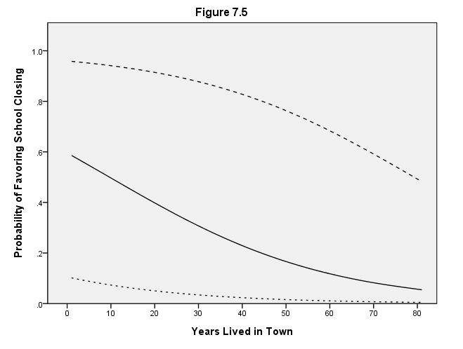
Page 232 Figure 7.5 Conditional effects of years lived in town, at proclosing (top), average, and anticlosing levels of other X variables.
LOGISTIC REGRESSION VAR=close
  /METHOD=ENTER lived educ contam hsc nodad.
| Unweighted Cases(a) | N | Percent | |
|---|---|---|---|
| Selected Cases | Included in Analysis | 153 | 100.0 |
| Missing Cases | 0 | .0 | |
| Total | 153 | 100.0 | |
| Unselected Cases | 0 | .0 | |
| Total | 153 | 100.0 | |
| a If weight is in effect, see classification table for the total number of cases. | |||
| Original Value | Internal Value |
|---|---|
| open | 0 |
| close | 1 |
| |
Predicted | ||||
|---|---|---|---|---|---|
| schools should close | Percentage Correct | ||||
| Observed | open | close | |||
| Step 0 | schools should close | open | 87 | 0 | 100.0 |
| close | 66 | 0 | .0 | ||
| Overall Percentage | |
|
56.9 | ||
| a Constant is included in the model. | |||||
| b The cut value is .500 | |||||
| |
B | S.E. | Wald | df | Sig. | Exp(B) | |
|---|---|---|---|---|---|---|---|
| Step 0 | Constant | -.276 | .163 | 2.864 | 1 | .091 | .759 |
| |
Score | df | Sig. | ||
|---|---|---|---|---|---|
| Step 0 | Variables | LIVED | 12.683 | 1 | .000 |
| EDUC | .221 | 1 | .638 | ||
| CONTAM | 17.292 | 1 | .000 | ||
| HSC | 39.337 | 1 | .000 | ||
| NODAD | 9.835 | 1 | .002 | ||
| Overall Statistics | 56.279 | 5 | .000 | ||
| |
Chi-square | df | Sig. | |
|---|---|---|---|---|
| Step 1 | Step | 66.559 | 5 | .000 |
| Block | 66.559 | 5 | .000 | |
| Model | 66.559 | 5 | .000 | |
| Step | -2 Log likelihood | Cox & Snell R Square | Nagelkerke R Square |
|---|---|---|---|
| 1 | 142.652 | .353 | .473 |
| |
Predicted | ||||
|---|---|---|---|---|---|
| schools should close | Percentage Correct | ||||
| Observed | open | close | |||
| Step 1 | schools should close | open | 76 | 11 | 87.4 |
| close | 25 | 41 | 62.1 | ||
| Overall Percentage | |
|
76.5 | ||
| a The cut value is .500 | |||||
| |
B | S.E. | Wald | df | Sig. | Exp(B) | |
|---|---|---|---|---|---|---|---|
| Step 1(a) | LIVED | -.040 | .015 | 6.559 | 1 | .010 | .961 |
| EDUC | -.197 | .093 | 4.509 | 1 | .034 | .821 | |
| CONTAM | 1.298 | .477 | 7.422 | 1 | .006 | 3.664 | |
| HSC | 2.278 | .490 | 21.590 | 1 | .000 | 9.762 | |
| NODAD | -1.731 | .725 | 5.695 | 1 | .017 | .177 | |
| Constant | 2.182 | 1.330 | 2.691 | 1 | .101 | 8.865 | |
| a Variable(s) entered on step 1: LIVED, EDUC, CONTAM, HSC, NODAD. | |||||||
SORT CASES BY
  lived (A).

compute lhat1 = 3.17-.04*lived.
compute phat1 = 1/(1+exp(-lhat1)).
compute lhat2 = .387-.04*(lived).
compute phat2 = 1/(1+exp(-lhat2)).
compute lhat3 = -2.14-.04*(lived).
compute phat3 = 1/(1+exp(-lhat3)).
execute.

formats lived (f2.0) phat1 phat2 phat3 (f2.1).
GGRAPH
  /GRAPHDATASET NAME="graphdataset" VARIABLES=lived phat1 phat2 phat3
  /GRAPHSPEC SOURCE=INLINE.
BEGIN GPL
SOURCE: s=userSource(id("graphdataset"))
DATA: lived=col(source(s), name("lived"))
DATA: phat1=col(source(s), name("phat1"))
DATA: phat2=col(source(s), name("phat2"))
DATA: phat3=col(source(s), name("phat3"))
GUIDE: text.title( label( "Figure 7.5" ) )
GUIDE: axis(dim(1), label("Years Lived in Town"), delta(10))
GUIDE: axis(dim(2), label("Probability of Favoring School Closing"), delta(.2))
SCALE: linear(dim(1), min(0), max(80))
SCALE: linear(dim(2), min(0), max(1))
ELEMENT: line(position(smooth.spline(lived*phat1)), shape(shape.dash))
ELEMENT: line(position(smooth.spline(lived*phat2)))
ELEMENT: line(position(smooth.spline(lived*phat3)), shape(shape.half_dash))
END GPL.
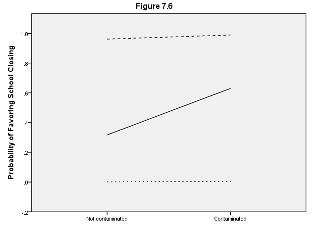
Page 232 Figure 7.6 Conditional effects of contamination, at proclosing, average, and anticlosing levels of other X variables.
SORT CASES BY contam (A).
compute lhat4 = 3.22+1.3*(contam).
compute phat4 = 1/(1+exp(-lhat4)).
compute lhat5 = -.7681+1.3*(contam).
compute phat5 = 1/(1+exp(-lhat5)).
compute lhat6 = -6.79+1.3*(contam).
compute phat6 = 1/(1+exp(-lhat6)).
execute.

SORT CASES BY
  contam (A).

value labels contam 0 "Not contaminated" 1 "Contaminated".
formats contam (f1.0) phat4 phat5 phat6 (f2.1).
GGRAPH
  /GRAPHDATASET NAME="graphdataset" VARIABLES=contam phat4 phat5 phat6
  /GRAPHSPEC SOURCE=INLINE.
BEGIN GPL
SOURCE: s=userSource(id("graphdataset"))
DATA: contam=col(source(s), name("contam"), unit.category() )
DATA: phat4=col(source(s), name("phat4"))
DATA: phat5=col(source(s), name("phat5"))
DATA: phat6=col(source(s), name("phat6"))
GUIDE: text.title( label( "Figure 7.6" ) )
GUIDE: axis(dim(1), label(" "))
GUIDE: axis(dim(2), label("Probability of Favoring School Closing"), delta(.2))
SCALE: linear(dim(2), min(-.2), max(1))
ELEMENT: line(position(smooth.spline(contam*phat4)), shape(shape.dash))
ELEMENT: line(position(smooth.spline(contam*phat5)))
ELEMENT: line(position(smooth.spline(contam*phat6)), shape(shape.half_dash))
END GPL.
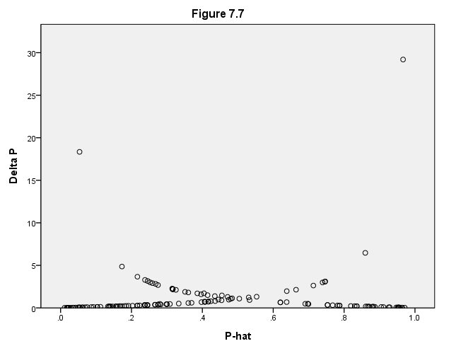
Page 239 Figure 7.7 Poorness-of-fit statistic delta-chi-square(P) versus predicted probability of favoring closed schools; X patterns 131 and 3 are poorly fit (high delta-chi-square(P) values).
LOGISTIC REGRESSION VAR=close
  /METHOD=ENTER lived educ contam hsc nodad
  /SAVE PRED COOK LEVER ZRESID DEV.
| Unweighted Cases(a) | N | Percent | |
|---|---|---|---|
| Selected Cases | Included in Analysis | 153 | 100.0 |
| Missing Cases | 0 | .0 | |
| Total | 153 | 100.0 | |
| Unselected Cases | 0 | .0 | |
| Total | 153 | 100.0 | |
| a If weight is in effect, see classification table for the total number of cases. | |||
| Original Value | Internal Value |
|---|---|
| open | 0 |
| close | 1 |
| |
Predicted | ||||
|---|---|---|---|---|---|
| schools should close | Percentage Correct | ||||
| Observed | open | close | |||
| Step 0 | schools should close | open | 87 | 0 | 100.0 |
| close | 66 | 0 | .0 | ||
| Overall Percentage | |
|
56.9 | ||
| a Constant is included in the model. | |||||
| b The cut value is .500 | |||||
| |
B | S.E. | Wald | df | Sig. | Exp(B) | |
|---|---|---|---|---|---|---|---|
| Step 0 | Constant | -.276 | .163 | 2.864 | 1 | .091 | .759 |
| |
Score | df | Sig. | ||
|---|---|---|---|---|---|
| Step 0 | Variables | LIVED | 12.683 | 1 | .000 |
| EDUC | .221 | 1 | .638 | ||
| CONTAM | 17.292 | 1 | .000 | ||
| HSC | 39.337 | 1 | .000 | ||
| NODAD | 9.835 | 1 | .002 | ||
| Overall Statistics | 56.279 | 5 | .000 | ||
| |
Chi-square | df | Sig. | |
|---|---|---|---|---|
| Step 1 | Step | 66.559 | 5 | .000 |
| Block | 66.559 | 5 | .000 | |
| Model | 66.559 | 5 | .000 | |
| Step | -2 Log likelihood | Cox & Snell R Square | Nagelkerke R Square |
|---|---|---|---|
| 1 | 142.652 | .353 | .473 |
| |
Predicted | ||||
|---|---|---|---|---|---|
| schools should close | Percentage Correct | ||||
| Observed | open | close | |||
| Step 1 | schools should close | open | 76 | 11 | 87.4 |
| close | 25 | 41 | 62.1 | ||
| Overall Percentage | |
|
76.5 | ||
| a The cut value is .500 | |||||
| |
B | S.E. | Wald | df | Sig. | Exp(B) | |
|---|---|---|---|---|---|---|---|
| Step 1(a) | LIVED | -.040 | .015 | 6.559 | 1 | .010 | .961 |
| EDUC | -.197 | .093 | 4.509 | 1 | .034 | .821 | |
| CONTAM | 1.298 | .477 | 7.422 | 1 | .006 | 3.664 | |
| HSC | 2.278 | .490 | 21.590 | 1 | .000 | 9.762 | |
| NODAD | -1.731 | .725 | 5.695 | 1 | .017 | .177 | |
| Constant | 2.182 | 1.330 | 2.691 | 1 | .101 | 8.865 | |
| a Variable(s) entered on step 1: LIVED, EDUC, CONTAM, HSC, NODAD. | |||||||
compute deltap=(zre_1)**2/(1-lev_1).
execute.

formats pre_1 (f2.1) deltap (f2.0).
GGRAPH
  /GRAPHDATASET NAME="graphdataset" VARIABLES=pre_1 deltap
  /GRAPHSPEC SOURCE=INLINE.
BEGIN GPL
SOURCE: s=userSource(id("graphdataset"))
DATA: deltap=col(source(s), name("deltap"))
DATA: pre_1=col(source(s), name("pre_1"))
GUIDE: text.title( label( "Figure 7.7" ) )
GUIDE: axis(dim(1), label("P-hat"), delta(.2))
GUIDE: axis(dim(2), label("Delta P"), delta(5))
SCALE: linear(dim(1), min(0), max(1))
SCALE: linear(dim(2), min(0), max(30))
ELEMENT: point(position(pre_1*deltap))
END GPL.
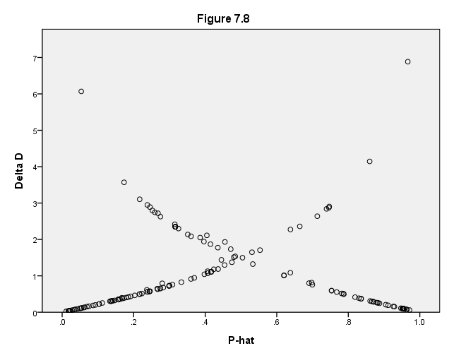
Page 240 Figure 7.8 Poorness-of-fit statistic delta-chi-square(D) versus predicted probability of favoring closed schools; X patterns 131, 3, 27, 62, 115 are poorly fit (high delta-chi-square(D) values).
compute deltad=(dev_1)**2/(1-lev_1).
execute.

formats deltad (f2.0).
GGRAPH
  /GRAPHDATASET NAME="graphdataset" VARIABLES=pre_1 deltad
  /GRAPHSPEC SOURCE=INLINE.
BEGIN GPL
SOURCE: s=userSource(id("graphdataset"))
DATA: deltad=col(source(s), name("deltad"))
DATA: pre_1=col(source(s), name("pre_1"))
GUIDE: text.title( label( "Figure 7.8" ) )
GUIDE: axis(dim(1), label("P-hat"), delta(.2))
GUIDE: axis(dim(2), label("Delta D"), delta(1))
SCALE: linear(dim(1), min(0), max(1))
SCALE: linear(dim(2), min(0), max(7))
ELEMENT: point(position(pre_1*deltad))
END GPL.
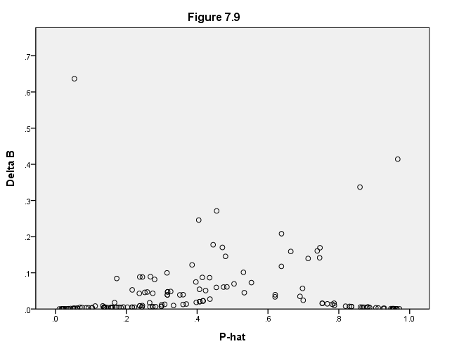
Page 241 Figure 7.9 Influence statistic delta-B versus predicted probability of favoring closed schools; patterns 131, 3, 115, 44, and 94 are most influential (high delta-B values).
NOTE: Delta-B is the Cook’s D statistic.
formats coo_1 (f2.1).
GGRAPH
  /GRAPHDATASET NAME="graphdataset" VARIABLES=pre_1 coo_1
  /GRAPHSPEC SOURCE=INLINE.
BEGIN GPL
SOURCE: s=userSource(id("graphdataset"))
DATA: coo_1=col(source(s), name("coo_1"))
DATA: pre_1=col(source(s), name("pre_1"))
GUIDE: text.title( label( "Figure 7.9" ) )
GUIDE: axis(dim(1), label("P-hat"), delta(.2))
GUIDE: axis(dim(2), label("Delta B"), delta(.1))
SCALE: linear(dim(1), min(0), max(1))
SCALE: linear(dim(2), min(0), max(.7))
ELEMENT: point(position(pre_1*coo_1))
END GPL.
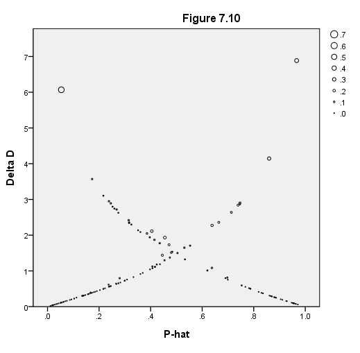
Page 242 Figure 7.10 Delta-chi-square(D) versus P-hat with
symbols proportional to delta-B; large, high circles indicate influential, poorly fit X
patterns.
GGRAPH
  /GRAPHDATASET NAME="graphdataset" VARIABLES=pre_1 deltad coo_1
  /GRAPHSPEC SOURCE=INLINE.
BEGIN GPL
SOURCE: s=userSource(id("graphdataset"))
DATA: deltad=col(source(s), name("deltad"))
DATA: pre_1=col(source(s), name("pre_1"))
DATA: coo_1=col(source(s), name("coo_1"))
GUIDE: text.title( label( "Figure 7.10" ) )
GUIDE: axis(dim(1), label("P-hat"), delta(.2))
GUIDE: axis(dim(2), label("Delta D"), delta(1))
SCALE: linear(dim(1), min(0), max(1))
SCALE: linear(dim(2), min(0), max(7))
ELEMENT: point(position(pre_1*deltad), size(coo_1))
END GPL.