When analyzing longitudinal data, we often want to know the first and last non-missing value of a variable that is measured repeatedly over time for each unit (e.g. patient, subject). For example, for a survival analysis we might want to capture a patient’s status (e.g. alive or dead) at the time of the first and last observations of that patient, where those times may vary across patients.
We present methods here to capture the first and last non-missing value of a variable, as well as the timing of those values, separately by id, for longitudinal data stored in two different formats.
Data in long format
When longitudinal data are in long format, each unit (person, subject) will have several rows of data, and the repeated measurements of a variable will typically be contained in a single variable (column).
Here we use the DATA LIST command to create a small example data set that contains the following variables:
- id: subject id
- time: time point
- Y: variable for which we want the first and last values
DATA LIST LIST
/id time Y.
BEGIN DATA.
1, 1, 5
1, 2, 4
1, 3,
1, 4,
1, 5, 7
2, 1,
2, 2,
2, 3, 1
2, 4, 3
2 ,5, 2
3, 1,
3, 2, 4,
3, 3,
3, 4, 3
3, 5,
4, 1,
4, 2,
4, 3,
4, 4,
4, 5
END DATA.
We have purposely included a subject that has all missing values (subject 4) to demonstrate what this code will do in such cases.
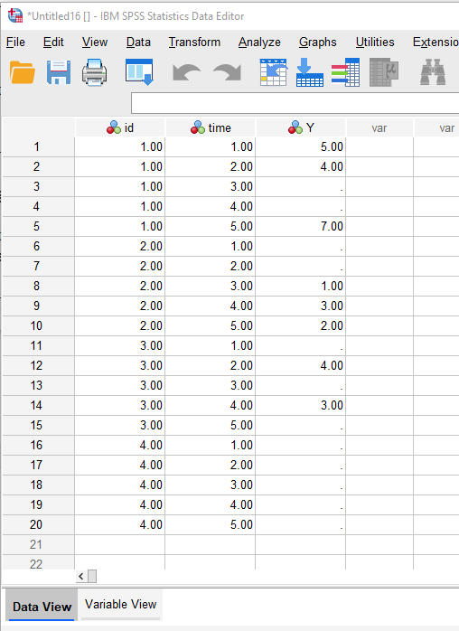
If you have entered the DATA LIST command, you should see the data in SPSS like this:
GOAL: Our goal is to capture the first and last non-missing values of the Y variable for each id, as well as the timing of the first and last values. For example, for subject 2, we want the capture the first non-missing Y value, 1, which occurs at time=3, and the last non-missing Y value, 2, which occurs at time=5.
STRATEGY: Our general strategy consists of the following steps:
- Create a filter that will filter out observations missing on Y and apply that filter.
- Use the AGGREGATE command to capture the first and last observations of Y, which will now include only non-missing values after turning on the filter.
- Turn off the filter.
We use SPSS syntax to accomplish these tasks, but will also point out how to use the SPSS menus to accomplish the same tasks.
Step 1: Create and apply a filter that filters out observations missing on Y.
In the syntax below, the COMPUTE command creates a filter variable, filter_$, that equals 1 if the observation is not missing on Y and equals 0 if the observation is missing on Y. The subsequent FILTER command then tells SPSS to only use observations where filter_$=1.
COMPUTE filter_$=(not missing(Y)).
FILTER BY filter_$.
EXE.

If using SPSS menus:
- Select Data > Select Cases
- Click the button If condition is satisfied
- Click the If button
- In the empty box, type “not missing(Y)”, where Y is the name of the variable whose last and first values you’re capturing
- Click Continue
- Click OK
Step 2: Use the AGGREGATE command to capture the first and last values of Y
The syntax below runs the AGGREGATE command, which processes data by a “break variable”, here id. We create 2 new variables, Y_first and Y_last, to store the first and last values of Y by id.
AGGREGATE
  /OUTFILE=* MODE=ADDVARIABLES
  /BREAK=id
  /Y_first=FIRST(Y)
  /t_first=FIRST(time)
  /Y_last=LAST(Y)
  /t_last=LAST(time).
If using SPSS menus:
- Select Data > Aggregate
- Move the id variable to the “Break Variable(s)” box
- Move the Y variable to the “Summaries of Variable(s)” box
- Click the Function button
- Click the First button. Then click Continue.
- Move the Y variable to the “Summaries of Variable(s)” box again
- Click the Function button
- Click the Last button. Then click Continue.
- Repeat steps 3 through 8 for the time variable
- Click the OK button
Step 3: Turn the missing data filter off.
Syntax:
FILTER off.
EXE.
If using SPSS menus:
- Select Data > Select Cases
- Click the button All cases
Result
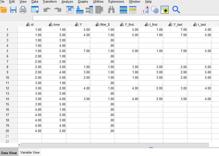
After following the steps above, the resulting data set will contain 2 new variables that capture the first and last non-missing observations of the Y variable, as well as the time of those observations:
Optional Step 4: If you need to fill in the missing values of the newly created variables, we provide syntax to accomplish this.
Syntax: The syntax below first sorts the data by time in descending order. It then checks whether there is missing value for a particular variable, and if so, checks if the row below has a non-missing value. If the next row has a non-missing value, the code copies that value into the current row. Then, we sort by time in ascending order and repeat the same process.
sort cases by id time(D).
if (lag(id) = id) & missing(Y_first) & not missing(lag(Y_first)) Y_first = lag(Y_first).
if (lag(id) = id) & missing(t_first) & not missing(lag(t_first)) t_first = lag(t_first).
if (lag(id) = id) & missing(Y_last) & not missing(lag(Y_last)) Y_last = lag(Y_last).
if (lag(id) = id) & missing(t_last) & not missing(lag(t_last)) t_last = lag(t_last).
exe.

sort cases by id time(A).
if (lag(id) = id) & missing(Y_first) & not missing(lag(Y_first)) Y_first = lag(Y_first).
if (lag(id) = id) & missing(t_first) & not missing(lag(t_first)) t_first = lag(t_first).
if (lag(id) = id) & missing(Y_last) & not missing(lag(Y_last)) Y_last = lag(Y_last).
if (lag(id) = id) & missing(t_last) & not missing(lag(t_last)) t_last = lag(t_last).
exe.
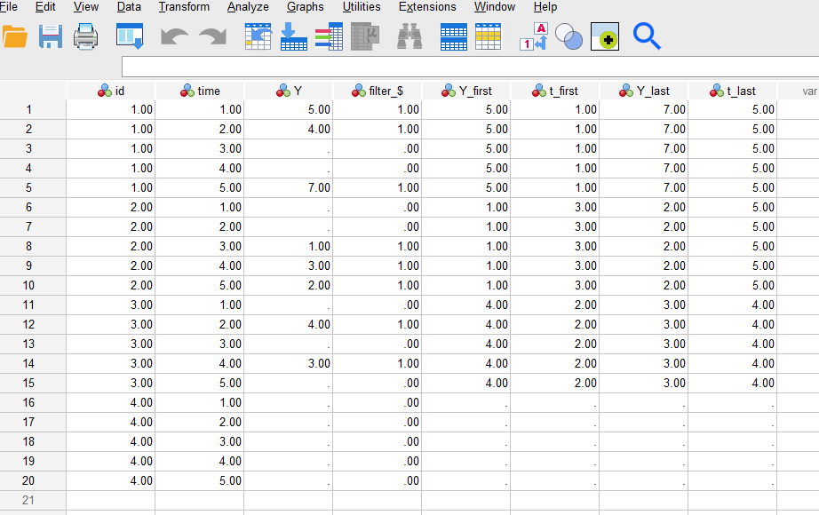
After running this optional step, these are the data:
Data in wide format
When longitudinal data are in wide format, repeated measurements of the same variable will be recorded in separate variables (columns).
Here we use the DATA LIST command again to create a small example wide data set that contains the following variables:
- id: subject id
- Y_t1, Y_t2, Y_t3, Y_t4, Y_t5: repeated measurements of variable Y over 5 time points
DATA LIST LIST
    /id Y_t1 Y_t2 Y_t3 Y_t4 Y_t5.
BEGIN DATA.
1, 5, 4, , , 7
2, , , 1, 3, 2
3, , 4, , 3,
4, , , , , ,
END DATA.
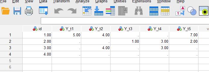
After running the DATA LIST command, the data should appear like this:
GOAL: Our goal is to capture the first and last non-missing values of the Y variable for each id, as well as the timing of the first and last values.
STRATEGY: Our general strategy consists of the following steps:
- Run LOOP commands to loop over the repeated measures variables, Y_t1, Y_t2, Y_t3, Y_t4, Y_t5. The LOOP command processes each row of data separately.
- First LOOP starting with Y_t1 and proceed forwards.
- Stop when we hit a non-missing value, and record the Y value and the value of the loop index variable, which represents the time of the measurement. These will be the first non-missing Y value and its timing.
- Then LOOP starting with Y_t5 and proceed backwards.
- Stop when we hit a non-missing value, and record the Y value and the value of the loop index variable, which represents the time of the measurement. These will be the last non-missing Y value and its timing.
- Fix the new time variables for cases that have missing on all repeated measurements (here, missing on all of Y_t1, Y_t2, Y_t3, Y_t4, Y_t5).
The LOOP command is not available through SPSS menus, so we only provide a syntax solution here.
Step 1: Run the LOOP commands to create the new variables.
In the syntax below, the VECTOR command is used to create a vector of variables that can be accessed using a numeric index. For example, “vector V = Y_t1 to Y_t5.” creates a vector of 5 variables, and we can access the contents of Y_t3 using V(3).
In the LOOP commands:
- We create a loop index variable, either t_first or t_last, which start at 1 and 5, respectively, and increment or decrement by 1, respectively.
- Each LOOP iterates over the vector of variables, V, and stops when it reaches the first non-missing value. In the second LOOP, where we start at the end and go backwards, the first non-missing value we encounter is the last non-missing value across Y_t1, Y_t2, Y_t3, Y_t4, Y_t5.
Here is the syntax:
* get first non-missing Y_t value.
vector V = Y_t1 to Y_t5.
loop t_first = 1 to 5 by 1.
end loop if not missing(V(t_first)).
compute Y_first = V(t_first).
exe.

* get last non-missing Y_t value.
vector V = Y_t1 to Y_t5.
loop t_last = 5 to 1 by -1.
end loop if not missing(V(t_last)).
compute Y_last =V(t_last).
exe.
Step 2: Set t_first and t_last to missing for cases with missing on all Y variables
If an observation has missing on all of the repeated measurements (here Y_t1, Y_t2, Y_t3, Y_t4, Y_t5), for example with id=4 above, we want the timing of those measurements, recorded in t_first and t_last, to be set to missing as well. This step is not necessary if there are no missing values in the repeated measurement variables.
Syntax:
if t_last < 1 t_last = $sysmis.
exe.

if t_first > 5 t_first = $sysmis.
exe.
Result:
After running the syntax in the 2 steps above, the resulting data are:


