Sometimes your research hypothesis may predict that the size of a regression coefficient should be bigger for one group than for another. For example, you might believe that the regression coefficient of height predicting weight would be higher for men than for women. Below, we have a data file with 10 fictional females and 10 fictional males, along with their height in inches and their weight in pounds.
data list free
 / id * gender (A8) height * weight.
begin data.
 1   F  56 117
 2   F  60 125
 3   F  64 133
 4   F  68 141
 5   F  72 149
 6   F  54 109
 7   F  62 128
 8   F  65 131
 9   F  65 131
10   F  70 145
11   M  64 211
12   M  68 223
13   M  72 235
14   M  76 247
15   M  80 259
16   M  62 201
17   M  69 228
18   M  74 245
19   M  75 241
20   M  82 269
end data.
execute.
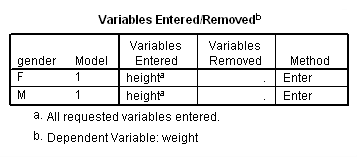
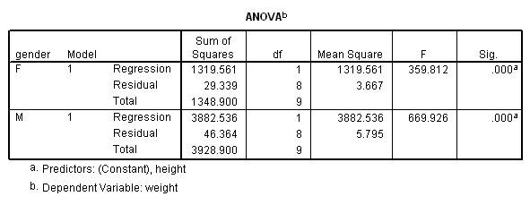
We analyzed their data separately using the regression commands below. Note that we have to do two regressions, one with the data for females only and one with the data for males only. We can use the split file command to split the data file by gender and then run the regression. The parameter estimates (coefficients) for females and males are shown below, and the results do seem to suggest that height is a stronger predictor of weight for males (3.18) than for females (2.09).
sort cases by gender.
split file by gender.
regression
 /dep weight
 /method = enter height.
split file off.
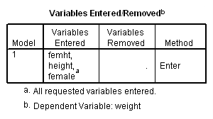
We can compare the regression coefficients of males with females to test the null hypothesis Ho: Bf = Bm, where Bf is the regression coefficient for females, and Bm is the regression coefficient for males. To do this analysis, we first make a dummy variable called female that is coded 1 for female and 0 for male, and a variable femht that is the product of female and height. We then use female, height and femht as predictors in the regression equation.
split file off.

compute female = 0.
if gender = "F" female = 1.
compute femht = female*height.
execute.

regression
 /dep weight
 /method = enter female height femht.
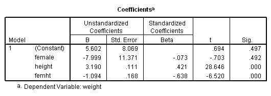
The output is shown below.
The term femht tests the null hypothesis Ho: Bf = Bm. The T value is -6.52 and is significant, indicating that the regression coefficient Bf is significantly different from Bm.
Let’s look at the parameter estimates to get a better understanding of what they mean and
how they are interpreted.
First, recall that our dummy variable
female is 1 if female and 0 if
male; therefore, males are the omitted group. This is needed for proper interpretation
of the estimates.
          Parameter
Variable  Estimate
INTERCEP  5.601677 : This is the intercept for the males (omitted group)
                     This corresponds to the intercept for males in
                     the separate groups analysis.
FEMALE   -7.999147 : Intercept Females - Intercept males
                     This corresponds to differences of the
                     intercepts from the separate groups analysis.
                     and is indeed -2.397470040 - 5.601677149
HEIGHT    3.189727 : Slope for males (omitted group), i.e. Bm.
FEMHT    -1.093855 : Slope for females - Slope for males
                     (i.e. Bf - Bm).
                     From the separate groups, this is indeed
                     2.095872170 - 3.189727463 .
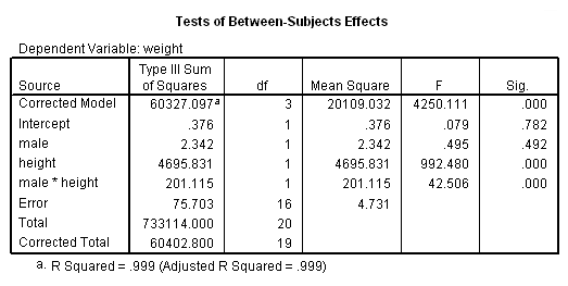
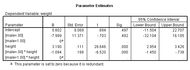
It is also possible to run such an analysis using glm, using syntax like that below. Note that other statistical packages, such as SAS and Stata, omit the group of the dummy variable that is coded as zero. However, SPSS omits the group coded as one. Therefore, when you compare the output from the different packages, the results seem to be different. To make the SPSS results match those from other packages, you need to create a new variable that has the opposite coding (i.e., switching the zeros and ones). We do this with the male variable. We do not know of an option in SPSS glm to easily change which group is the omitted group. (Please note that you can use the contrast subcommand to get the contrast coefficient for female using 0 as the reference group; however, the coding of female in the interaction is such that 1 is used as the reference group, so the use of the contrast subcommand is not very helpful in this situation.)
compute male = not female.glm weight by male with height /design = male height male by height /print = parameter.
As you see, the glm output corresponds to the output obtained by regression. The parameter estimates appear at the end of the glm output. They also correspond to the output from regression.

