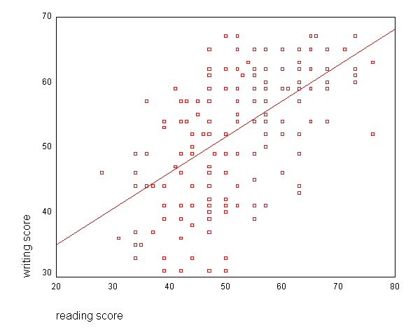
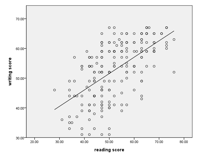
There are at least two ways to make a scatterplot with a regression line in SPSS. One way is to use the graph command, and another way is to use the ggraph command. Both are illustrated below.
Let’s read in an example dataset, hsb2, which contains data from the High School and Beyond study.
get file 'c:hsb2.sav'.
Let’s do a scatterplot of the variables write with read. Note that after running the code below, you need to double click on the graph, which will open up the chart editor window. Select "chart" from the menu at the top and then "options" (which is the first item in the menu). On the right of the dialogue box is a check box called "Total" under the heading "Fit Line". Click on the box to put in the check, or click on "Fit Options" to select a different type of fit method, such as lowess, quadratic or cubic. Close the chart editor so that the changes to take effect on your graph.
Using the graph command
graph
  /scatterplot(bivar)=read with write.

Using the ggraph command
The ggraph command was introduced in version 14 of SPSS. This command can be used to create and edit scatterplots. Below is the syntax for creating a scatterplot with the regression line.
GGRAPH
  /GRAPHDATASET NAME="graphdataset" VARIABLES=read write
  /GRAPHSPEC SOURCE=INLINE.
BEGIN GPL
 SOURCE: s=userSource(id("graphdataset"))
 DATA: read=col(source(s), name("read"))
 DATA: write=col(source(s), name("write"))
 GUIDE: axis(dim(1), label("reading score"))
 GUIDE: axis(dim(2), label("writing score"))
 ELEMENT: line( position( smooth.linear(read*write ) ) )
 ELEMENT: point(position(read*write))
END GPL.

