If you are not familiar with three-way interactions in ANOVA, please see our general FAQ on understanding three-way interactions in ANOVA. In short, a three-way interaction means that there is a two-way interaction that varies across levels of a third variable. Say, for example, that a b*c interaction differs across various levels of factor a.
One way of analyzing the three-way interaction is through the use of tests of simple main-effects, e.g., the effect of one variable (or set of variables) across the levels of another variable.
Next, we need to obtain the tests of the simple main-effects for each level of a. For this example, the residual mean-square is the error term for all of the effects in the model and thus, for all of the tests of simple main-effects. There are at least three ways to conduct these tests. Perhaps the easiest way is to simply do some calculations by hand. Another way to do this is to use the lmatrix subcommand and specify the various contrasts. Once you understand how to code the contrasts on the lmatrix subcommand, this is a simple method with minimal syntax required. An example illustrating this method can be found here. A third way to do this is to use OMS (Output Management System) to capture the necessary values and use aggregate to calculate the necessary values. The advantage of this method is that you can get the adjusted p-values and critical F values per family error rate; however, this requires some SPSS syntax that some people find intimidating. An example illustrating this method can be found here.
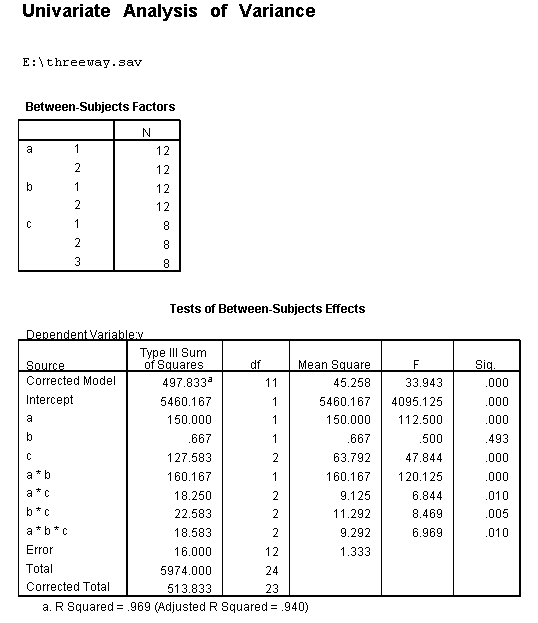
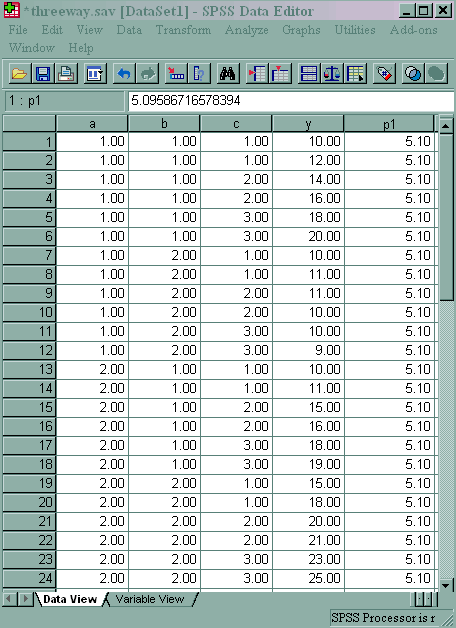
We will use a small artificial dataset called threeway that has a statistically significant three-way interaction to illustrate the process. In our example data set, variables a, b and c are categorical. The techniques shown on this page can be generalized to situations in which one or more variables are continuous, but the more continuous variables that are involved in the interaction, the more complicated things get.
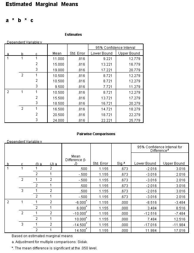
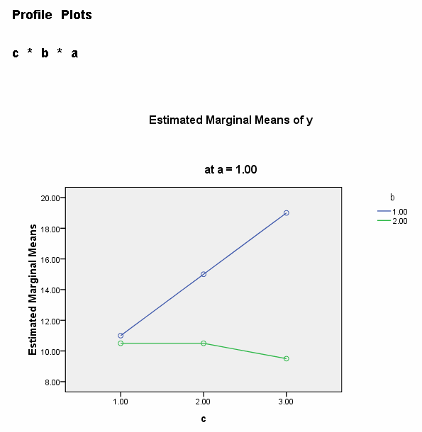
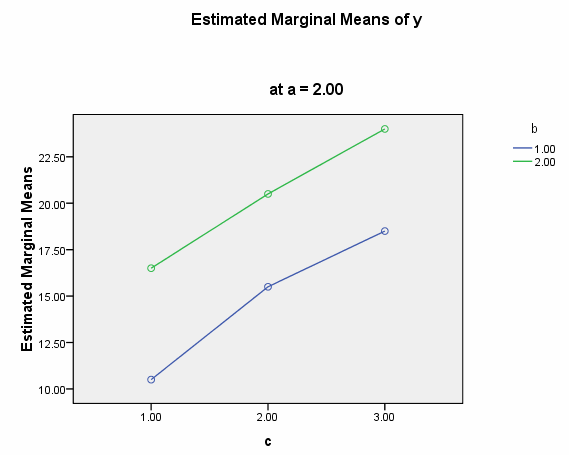
We need to select a two-way interaction to look at more closely. For the purposes of this example we will examine the b*c interaction. We can use the plot subcommand of the unianova command to graph the b*c interaction for each of the two levels of a. We use the emmeans subcommands to get the numeric values that are displayed on the graphs.
unianova y by a b c
/plot = profile(c*b*a)
/emmeans=tables(a*b*c)
/design = a b c a*b a*c b*c a*b*c.
We believe from looking at the two graphs above that the three-way interaction is significant because there appears to be a “strong” two-way interaction at a = 1 and no interaction at a = 2. Now, we just have to show it statistically using tests of simple main-effects.
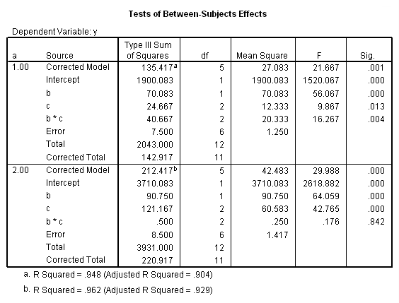
In SPSS, we need to conduct the tests of simple main-effects in two parts. First, we begin by running the ANOVA for both levels of a. This is easily done by sorting the data file on a, then splitting the file by a, running the ANOVA, and finally turning off the split file. To save space, we show only some of the output from the unianova command.
sort cases by a.
split file by a.
unianova y by b c
/design = b c b*c.
split file off.
Next, we need to obtain the tests of the simple main-effects for each level of a. For this example, the residual mean-square is the error term for all of the effects in the model and thus, for all of the tests of simple main-effects. Let’s rerun the model from above (with fewer subcommands so as to reduce the amount of output).
unianova y by a b c
/design = a b c a*b a*c b*c a*b*c.
As we can see, the sums of squares error is 16 with 12 degrees of freedom; the mean square error is 1.333.
Now, let’s look at the b*c interaction at a=1. The test statistic is obtained by dividing the mean square of the b*c interaction from the ANOVA with just b and c at a=1 by the mean square error from the original ANOVA. To do this, we need sort the data file by a, split the data file by a, and then run the ANOVA with b, c and the b*c interaction as predictors of y.
sort cases by a.
split file by a.
unianova y by b c.
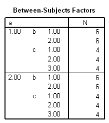

The mean square of the b*c interaction is 20.333. So we have 20.333/1.333 = 15.25. To test the b*c interaction at a=2, we have .250/1.333 = .1875. The first test, F(2, 12) = 15.25
Clearly, the first F-ratio, F(2, 12) = 15.25, is much larger than the second, F(2, 12) = .1875, but how can we tell which are statistically significant? There are at least four different methods of determining the critical value of tests of simple main-effects. There is a method related to Dunn’s multiple comparisons, a method attributed to Marascuilo and Levin, a method called the simultaneous test procedure (very conservative and related to the Scheffé post-hoc test) and a per family error rate method.
We will demonstrate the per family error rate method but you should look up the other methods in a good ANOVA book, like Kirk (1995), to decide which approach is best for your situation. We divide our alpha level, 0.05, by 2 because we are doing two tests of simple main-effects, so our new value of alpha is .025. The idf function requires us to provide 1 – alpha, so we have 1 – .025 = .975.
compute p1 = idf.f(.975, 2, 12).
exe.
As you can see, p1 is approximately 5.10. This indicates that the b*c interaction is statistically significant at a=1 but not at a=2.
In an ideal world we would be done now, but since we live in the “real” world, there is still more to do because we now need to try to understand the significant two-way interaction at a = 1; first for b = 1 and then for b = 2.
For a = 1 and b = 1:
compute filter1 = 0.
if b=1 and a = 1 filter1 = 1.
exe.

filter by filter1.
unianova y by c.
filter off.
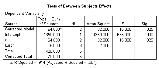
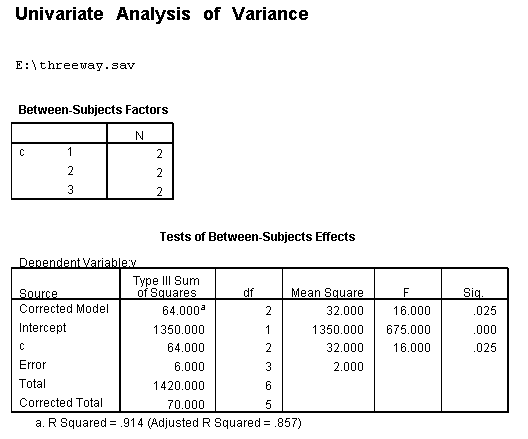
We will construct this F test in the same way we did above, namely using the mean square for the effect, in this case, the effect of c, divided by the mean square error from the original ANOVA. As we can see from the output above, the mean square for c is 32. Hence, we have 32/1.33 = 24. We can obtain the critical F-value using the idf function.
compute p1 = idf.f(.975, 2, 12).
exe.
The critical value is approximately 5.1, so our F(2, 12) = 24 is statistically significant.
For a = 1 and b = 2:
compute filter2 = 0.
if b=2 and a = 1 filter2 = 1.
exe.

filter by filter2.
unianova y by c.
filter off.
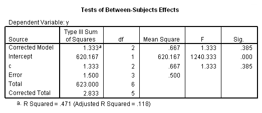
We will construct this F test in the same way we did above, namely using the mean square for the effect, in this case, the effect of c, divided by the mean square error from the original ANOVA. As we can see from the output above, the mean square for c is .667. Hence, we have .667/1.33 = .5. We can obtain the critical F-value using the idf function.
compute p2 = idf.f(.975, 2, 12).
exe.
The critical value is approximately 5.1, so our F(2, 12) = .5 is not statistically significant.
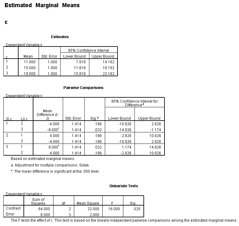
Only the test of simple main-effects of c at b = 1 was significant. But we’re not done yet, since there are three levels of c, we don’t know where this significant effect lies. We need to test the pairwise comparisons among the three means. We will do this using the Sidak correction for multiple tests.
filter by filter1.
unianova y by c
/emmeans=tables(c) compare(c) adj(sidak) .
filter off.
As shown above, only one of the comparisons is statistically significant. However, the Sidak correction can be conservative. If we had used a different correction, say the Tukey HSD, all three comparisons would be statistically significant. We should note that the error term used in these comparisons is not the error term from the original three-way ANOVA. We would need to use syntax similar to that shown above to save that error term to a new data set and then use it in the comparisons (as shown on https://stats.idre.ucla.edu/stat/stata/faq/threeway.htm ). We might want to use the error term from the original three-way ANOVA because we are going post-hoc tests of that analysis.
Hopefully, we now have a much better understanding of the three-way a*b*c interaction.
Please note that the process of investigating the three-way interactions would have be similar if we had chosen a different two-way interaction back at the beginning.
Summary of Steps
1) Run full model with three-way interaction. 1a) Capture SS and df residual. 2) Run two-way interaction at each level of third variable. 2a) Capture SS and df for interactions. 2b) Compute F-ratios for tests of simple main-effects. 3) Run one-way model at each level of second variable. 3a) Capture SS and df for main effects. 3b) Compute F-ratios for tests of simple main-effects. 4) Run pairwise or other post-hoc comparisons if necessary.
References
Kirk, Roger E. (1995) Experimental Design: Procedures for the Behavioral Sciences, Third Edition. Monterey, California: Brooks/Cole Publishing.

