Version info: The examples on this page were developed using SPSS version 21.
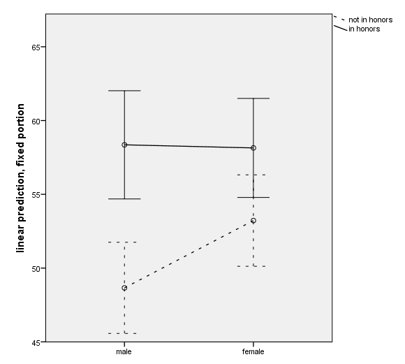
Let us suppose that you have data collected on children nested in schools. You have a continuous outcome variable, say scores on a writing test, and you run a multilevel model using the mixed command. Let us also suppose that you have two binary predictor variables, and you that would like to graph the estimated marginal means. You can get the estimated marginal means using the emmeans subcommand in the mixed command, but how do you get those values and their confidence intervals onto a graph?
To do this in SPSS, you will need to use OMS (Output Management System) to create a new dataset and the ggraph command. Before you use OMS, you should make sure that you have the model that you want to run, and that this model runs without errors. In our example, we will use the hsbdemo dataset. We will use the variable write as the outcome variable, and the binary variables female and honors as predictor variables. The level 2 identifier is called cid. We will have random intercepts for cid, but we will not include any random slopes. The syntax for our model is given below.
get file "D:datahsbdemo.sav".
dataset name hsbdemo.
dataset activate hsbdemo.
mixed write by female honors
/print = solution
/method = reml
/fixed = female honors female*honors
/random = intercept | subject(cid)
/emmeans = tables(female by honors).
The table from the output that we wish to make into a dataset is called Estimated Marginal Means. We will need this information for our oms command. We will also need to specify a location and name for our new data file. Our oms command will be followed by our mixed command, and that will be followed by the omsend command.
oms select tables
/destination  format = sav outfile = "D:Datamixed_marginsplot1.sav"
/if commands = ['mixed'] subtypes = [ 'Estimated Marginal Means'].

mixed write by female honors
/print = solution
/method = reml
/fixed = female honors female*honors
/random = intercept | subject(cid)
/emmeans = tables(female by honors).

omsend.
Now that we have created our new dataset, we can open the dataset and do some data management. We will use the autorecode command to make the string variables var1 and var2 into numeric variables. We will call these new numeric variables gender and hon, respectively. However, these variables are coded 1 and 2, rather than 0 and 1 as our original predictor variables were. We will use the recode command to create the variables female and honors. After adding value labels to these variables (which will be used in the graph), we will use the delete variables command to removed unneeded variables from our dataset.
get file "D:Datamixed_marginsplot1.sav".
dataset name mixed_marginsplot1.
dataset activate mixed_marginsplot1.

autorecode var = var1 var2 / into gender hon.
recode gender (2 = 0) (else = copy) into female.
value labels female 0 "male" 1 "female".
recode hon (2 =0) (else = copy) into honors.
value labels honors 0 "not in honors" 1 "in honors".
exe.
delete variables command_ subtype_ label_ gender hon.
Finally, we are ready to make our graph. We will use the ggraph command and list the variables needed to make the graph: mean, female, honors, upperbound and lowerbound. We use the inlinetemplate option on the graphspec subcommand to set the number of decimals shown on the y-axis to 0.
We need to use some GPL to add the elements to our graph. We use the SOURCE statement (which must be typed in capital letters) to identify the dataset to be used to make the graph. This name must match that given in the ggraph command. We use five DATA statements to define our five variables. Notice that female and honors as specified as categorical variables. We use a GUIDE statement to label the y-axis and to indicate that the values on the y-axis should increment in units of 5. The first SCALE statement indicates that the x-axis (called dim(1)) should include 0 and 1 (the variable female is coded 0 and 1). The second SCALE statement sets the minimum and maximum values for the scale on the y-axis. The first ELEMENT statement graphs the confidence intervals. The shape.interior function is used to specify the shape of the lines for the confidence intervals, and the shape.exterior function is used to specify different line types for the values of honors. The second ELEMENT statement graphs the means, and the third ELEMENT statement connects the means with lines.
ggraph
 /graphdataset name="GraphDataset" VARIABLES= mean female honors upperbound lowerbound
 /graphspec source = inline
inlinetemplate="<setTickLabelFormat categorical='false' role='y'><format minimumFractionDigits='0' maximumFractionDigits='0'/></setTickLabelFormat>".
BEGIN GPL
SOURCE: s=userSource( id( "GraphDataset" ) )
DATA: mean=col( source(s), name( "mean" ) )
DATA: female =col( source(s), name( "female" ), unit.category() )
DATA: honors = col(source(s), name("honors"), unit.category())
DATA: upperbound=col( source(s), name( "upperbound" ) )
DATA: lowerbound=col( source(s), name( "lowerbound" ) )
GUIDE: axis(dim(2), label("linear prediction, fixed portion"), delta(5))
SCALE: cat(dim(1), include("0", "1"))
SCALE: linear( dim( 2 ), min(45), max(65) )
ELEMENT: interval(position(region.spread.range(female*(lowerbound+upperbound))), shape.interior(shape.ibeam), shape.exterior(honors))
ELEMENT: point( position(female * mean))
ELEMENT: line(position(smooth.linear(female * mean)), shape(honors))
END GPL.

Example 2: Adding covariates to the model
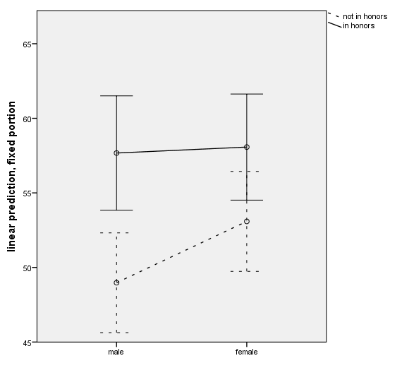
In this example, we will add two continuous predictor variables to our model. We will let SPSS hold these variables at their means when calculating the estimated marginal means, which is the default. The two covariates will be read and socst, which are scores on a reading test and on a social studies test. These have been included in the mixed command after the SPSS keyword with and on the fixed subcommand.
dataset activate hsbdemo.
oms select tables
/destination  format = sav outfile = "D:Datamixed_marginsplot2.sav"
/if commands = ['mixed'] subtypes = ['Estimated Marginal Means'].

mixed write by female honors with socst read
/print = solution
/method = reml
/fixed = female honors socst read female*honors
/random = intercept | subject(cid)
/emmeans = tables(female by honors).

omsend.

get file "D:Datamixed_marginsplot2.sav".
dataset name mixed_marginsplot2.
dataset activate mixed_marginsplot2.

autorecode var = var1 var2 / into gender hon.
recode gender (2 = 0) (else = copy) into female.
value labels female 0 "male" 1 "female".
recode hon (2 =0) (else = copy) into honors.
value labels honors 0 "not in honors" 1 "in honors".
exe.
delete variables command_ subtype_ label_ gender hon.

ggraph
 /graphdataset name="GraphDataset" VARIABLES= mean female honors upperbound lowerbound
 /graphspec source = inline
inlinetemplate="<setTickLabelFormat categorical='false' role='y'><format minimumFractionDigits='0' maximumFractionDigits='0'/></setTickLabelFormat>".
BEGIN GPL
SOURCE: s=userSource( id( "GraphDataset" ) )
DATA: mean=col( source(s), name( "mean" ) )
DATA: female =col( source(s), name( "female" ), unit.category() )
DATA: honors = col(source(s), name("honors"), unit.category())
DATA: upperbound=col( source(s), name( "upperbound" ) )
DATA: lowerbound=col( source(s), name( "lowerbound" ) )
GUIDE: axis(dim(2), label("linear prediction, fixed portion"), delta(5))
SCALE: cat(dim(1), include("0", "1"))
SCALE: linear( dim( 2 ), min(45), max(65) )
ELEMENT: interval(position(region.spread.range(female*(lowerbound+upperbound))), shape.interior(shape.ibeam), shape.exterior(honors))
ELEMENT: point( position(female * mean))
ELEMENT: line(position(smooth.linear(female * mean)), shape(honors))
END GPL.

Example 3: Holding covariates at a given value
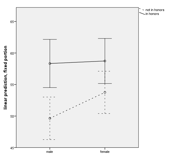
In this example, we will hold our covariates at specific, predefined values. We will hold the variable read at 50 and socst at 55. This has been added to the emmeans subcommand in the mixed command.
dataset activate hsbdemo.

oms select tables
/destination  format = sav outfile = "D:Datamixed_marginsplot3.sav"
/if commands = ['mixed'] subtypes = ['Estimated Marginal Means'].

mixed write by female honors with socst read
/print = solution
/method = reml
/fixed = female honors socst read female*honors
/random = intercept | subject(cid)
/emmeans = tables(female by honors) with(read = 50 socst = 55).

omsend.

get file "D:Datamixed_marginsplot3.sav".
dataset name mixed_marginsplot3.
dataset activate mixed_marginsplot3.

autorecode var = var1 var2 / into gender hon.
recode gender (2 = 0) (else = copy) into female.
value labels female 0 "male" 1 "female".
recode hon (2 =0) (else = copy) into honors.
value labels honors 0 "not in honors" 1 "in honors".
exe.
delete variables command_ subtype_ label_ gender hon.

ggraph
  /graphdataset name ="GraphDataset" VARIABLES= mean female honors upperbound lowerbound
 /graphspec source = inline
inlinetemplate="<setTickLabelFormat categorical='false' role='y'><format minimumFractionDigits='0' maximumFractionDigits='0'/></setTickLabelFormat>".
BEGIN GPL
SOURCE: s=userSource( id( "GraphDataset" ) )
DATA: mean=col( source(s), name( "mean" ) )
DATA: female =col( source(s), name( "female" ), unit.category() )
DATA: honors = col(source(s), name("honors"), unit.category())
DATA: upperbound=col( source(s), name( "upperbound" ) )
DATA: lowerbound=col( source(s), name( "lowerbound" ) )
GUIDE: axis(dim(2), label("linear prediction, fixed portion"), delta(5))
SCALE: cat(dim(1), include("0", "1"))
SCALE: linear( dim( 2 ), min(45), max(65) )
ELEMENT: interval(position(region.spread.range(female*(lowerbound+upperbound))), shape.interior(shape.ibeam), shape.exterior(honors))
ELEMENT: point( position(female * mean))
ELEMENT: line(position(smooth.linear(female * mean)), shape(honors))
END GPL.

